
SHAPE PRIOR SEGMENTATION OF MEDICAL IMAGES USING
PARTICLE SWARM OPTIMIZATION
Ahmed Afifi, Toshiya Nakaguchi and Norimichi Tsumura
Graduate School of Advanced Integration Science, Chiba University
1-33, Yayoi-cho, Inage-ku, Chiba-shi, Chiba, 263-8522, Japan
Keywords: Liver segmentation, Shape prior segmentation, Optimization for segmentation.
Abstract: The image segmentation is the first and essential process in many medical applications. This process is
traditionally performed by radiologists or medical specialists to manually trace the objects on each image. In
almost all of these applications, the medical specialists have to access a large number of images which is a
tedious and a time consuming process. On the other hand, the automatic segmentation is still challenging
because of low image contrast and ill-defined boundaries. In this work, we propose a fully automated
medical image segmentation framework. In this framework, the segmentation process is constrained by two
prior models; a shape prior model and a texture prior model. The shape prior model is constructed from a set
of manually segmented images using the principle component analysis (PCA) while the wavelet packet
decomposition is utilized to extract the texture features. The fisher linear discriminate algorithm is
employed to build the texture prior model from the set of texture features and to perform a preliminary
segmentation. Furthermore, the particle swarm optimization algorithm (PSO) is used to refine the
preliminary segmentation according to the shape prior model. In this work, we tested the proposed
technique for the segmentation of the liver from abdominal CT scans and the obtained results show the
efficiency of the proposed technique to accurately delineate the desired objects.
1 INTRODUCTION
The automatic segmentation of medical images is
very essential in almost all medical sites. And
consequently several methods have been developed
for this purpose (Bankman, 2000), (Dzung,
Chenyang, and Jerry, 2000). The traditional methods
utilize the intensity changes in order to extract the
edges and the local features of the desired objects
(Chi and Wang, 2000) or they start with a seed point
inside the region of interest and then grow the region
by using the similarity measures (Pan and Lu, 2007),
(Pohel and Toennies,2001). Despite these methods
are helpful in some situations, they are in adequate
for medical applications due to the existence of
noise, clutter, occlusion and the similarity between
objects intensity.
More advanced and a state of the art methods
model the segmentation problem as an optimization
of energy function (Mcinereny and Terzopoulos,
1996). In these methods, a closed curve deforms
until the balance is reached between the internal and
the external energy. This curve is represented as a
set of control points (Kass, Witkin, and Terzopoulos,
1988) or it is embedded as a zero level in a level set
function (Osher and Fedkiw, 2003). Although these
methods are more accurate than the traditional
methods, the reliance on image information only
usually leads to inaccurate results. The inclusion of
prior information has shown to improve the
segmentation results and recently there is an
increased interest in the methods relying on prior
information.
In this work, we propose an automated medical
image segmentation framework incorporating both
shape and texture prior. In this framework the
desired texture is efficiently modelled using the
over-complete wavelet packet decomposition. In
addition, a prior shape model is constructed by the
statistical analysis of a set of training shapes
describing the variation in object shape. The particle
swarm optimization algorithm (PSO) is used to
accurately segment the image by adapting the prior
shape model according to image features.
After this introduction, In Section2, we will
briefly introduce the particle swarm optimization
algorithm. In Section3, the proposed segmentation
framework will be described deeply. The
experimental results will be presented in Section4
291
Afifi A., Nakaguchi T. and Tsumura N. (2010).
SHAPE PRIOR SEGMENTATION OF MEDICAL IMAGES USING PARTICLE SWARM OPTIMIZATION.
In Proceedings of the 2nd International Conference on Agents and Artificial Intelligence - Artificial Intelligence, pages 291-297
DOI: 10.5220/0002724402910297
Copyright
c
SciTePress
and the paper will be concluded in Section5.
2 PARTICLE SWARM
OPTIMIZATION
PSO is a population based stochastic optimization
algorithm founded by Kennedy and Eberhart (1995)
. In this algorithm they mimic the social behaviour
of bird flocks searching for food to produce
computational intelligence. There are many
similarities between PSO and the other evolutionary
computation techniques, but PSO can achieve better
results in a faster, cheaper way compared to other
methods (Hassan, Cohanim, and Weck, 2005) .
In PSO, a population or swarm of individuals –
particles – are spread over the search space of some
problems. Each particle represents a complete
solution of this problem and it evaluates the
objective function at its location. The particle moves
in the search space under the influence of its
behaviour and the whole swarm behaviour.
Each particle in the swarm is defined by three d-
dimensional vectors; the current location
, the
velocity
and the best position it reaches
, where
d is the dimensionality of the search space. The
original PSO algorithm has been received many
enhancements from its appearance till now (Poli,
Kennedy, and Blackwell, 2007). The PSO with
inertia weight (Clerc, 2006) is one from these
enhancements which provides better control on the
search space and accordingly, we are interested in it
during this work. The PSO algorithm with inertia
weight will be described in the following algorithm.
1. Initialize the population array of particles with
random position and velocities.
Loop
2. For each particle, evaluate the desired
optimization objective function.
3. Comparing particle’s fitness evaluation with
its
, where
is the fitness evaluation
at particle’s best location. If current value is better
than
, then set
equal to the current
value, and
equal to the current location
.
4. Identifying the particle in the neighborhood with
the best success so far, and assign its index to
variable .
5. Changing the velocity and position of the particle
according to the following equations.
0,
0,
,
is the inertia weight
(1)
(2)
where:
• t refers to the iteration index.
•
0,
represents a vector of random
values uniformly distributed in
0,
.
• is a component-wise multiplication
•
is kept within the range
,
.
6. If a criterion is met (sufficiently good fitness or
maximum number of iteration), exit loop and
produce the output.
End loop
The researchers have found that the large value of
allows the particles to perform extensive exploration
and the small value of increases the chance to get
local optima. So they have found that the best
performance could be achieved by using a large
value of (e.g., 0.9) at the beginning and gradually
decrease it until reach another small value of ω.
3 THE PROPOSED
FRAMEWORK
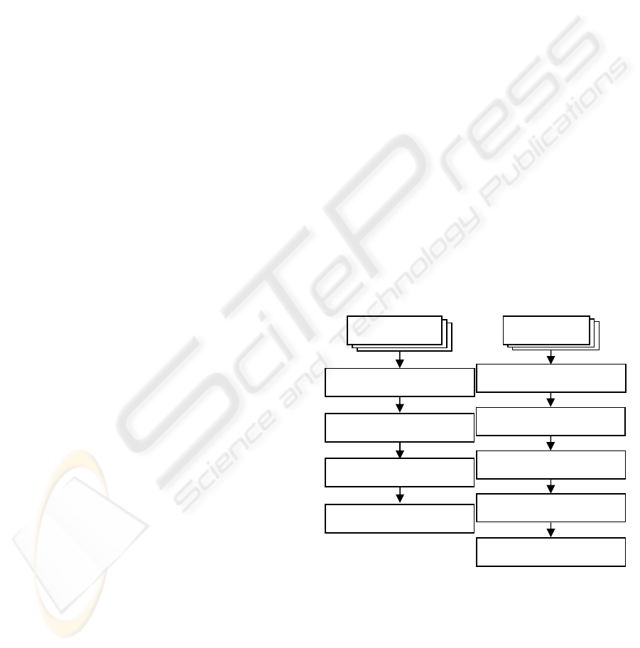
The proposed segmentation framework consists of
two stages; offline training and online segmentation
as shown in Figure1 and as we will demonstrate in
the following sections.
(a) (b)
Figure 1: The proposed framework, (a) The offline
training stage and (b) The online segmentation stage.
3.1 The Training Stage
3.1.1 Shape Alignment Model
In this work we are interested in aligning binary
New Images
Extract the Wavelet- features
Load the Prior Shape Model
Labelling each image pixel as a
desired object or not
Using the PSO Algorithm to fit the
Shape Model to the labelled image
Segment the Image According
to the Shape Model Parameters
Training
Images
Manual Segmentation and
Level Set Function Formulation
Prior Shape Model Formulation
Prior Texture Model Extraction
Shape Alignment
ICAART 2010 - 2nd International Conference on Agents and Artificial Intelligence
292

images with a value of one inside the object and a
value of zero outside. Let we have a training set
contains images
,
,…,
, the goal is to
calculate the set of pose parameters used to jointly
align the binary images. These parameters are
defined as ,,, and they represent the
,translation, scaling, rotation respectively. The
transformed image of , based on these pose
parameters, is denoted by
, and it is defined as
,
,
,
(3)
,
cos sin
,
sin cos
(4)
An effective strategy to jointly align the binary
images is to minimize the following energy
functional as defined in [15]:
Ω
Ω
,
(5)
where denotes the image domain. Minimizing (5)
is equivalent to simultaneously minimizing the
difference between any pair of binary images in the
training database. The area normalization term in the
denominator of (5) is employed to prevent all the
images from shrinking to improve the cost function.
Unlike the gradient descent employed in (Tasi et
al., 2003), the PSO algorithm can converge to almost
global minima. Therefore, in this work we utilize the
PSO algorithm to efficiently minimize that energy
function as described in the following algorithm.
1. Calculating the mean shape of the training
images.
2. Aligning every image to the mean shape using
PSO algorithm with a particles constructed from
,,,
and (5) as the objective function.
3. Calculating the mean shape of the aligned
images and if it is the same as the previous one,
end and produce the aligned images; else, go to
step2.
To illustrate this alignment process it is applied to a
set of 34 binary images of the liver and the
overlapping of these images before and after the
alignment is shown in Figure2.
3.1.2 Prior Shape Model Formulation
Motivated by the pioneering work of Tasi et al.
(2003), we derive the prior shape model from a set
of training images according to the following
algorithm.
(a) (b)
Figure 2: The amount of shape overlapping in the live
r
dataset (a) before alignment and (b) after alignment.
1. Deriving the level set functions that describe the
desired object from the n training images and
denote it as
,
,1,2,…,.
2. Computing the mean level set function
from
the set of level set functions
as
,
1
,
(6)
3. Deriving the shape variability function
according to equation (7).
,
,
(7)
4. Constructing a column vectors
,1,2,…,
consisting of samples of each
,
is the image size, by stacking the
columns
of
.
5. Defining the shape variability matrix S
as
…
.
6. Employing the Eigenvalue decomposition to the
shape variability matrix to compute the
variance in shape according to equation (8)
1
Σ
,
(8)
where is matrix whose columns
represent the n orthogonal modes of variation in
shapes and Σ
,
,…,
is an
diagonal matrix whose diagonals elements
represent the corresponding Eigenvalues.
7. Arranging back the N elements of each column
of to yield a maximum of n Eigenshapes or
principle modes
,1,2,…,.
3.1.3 Prior Texture Model Extraction
We utilize the over-complete wavelet packet
transform (Wang and Feng, 2005) to extract the
high-level feature vectors for each pixel in the
training images. The over-complete wavelet packet
transform doesn’t perform the down-sampling as in
SHAPE PRIOR SEGMENTATION OF MEDICAL IMAGES USING PARTICLE SWARM OPTIMIZATION
293

standard wavelet packet transform, so it ensures the
translation invariance property which is
indispensable for textural analysis. In addition, it
provides robust texture features at the expense of
redundancy (Li et al, 2005). In this work, we extract
the wavelet packet feature set by employing the
following algorithm.
1. Applying a two-level over-complete wavelet
packet decomposition on the input image.
2. At level-1, select the four sub-bands as feature
sub-images.
3. At level-2, in each sub-channel, selecting the
sub-band with the maximum variance to be a
feature sub-image.
4. Calculating the local energy around each pixel
of the feature sub-images as
,
1
2 1
,
(9)
where
,
is the wavelet coefficient
of a feature sub-image in the
2 1
2
1 window centered at pixel
,
.
5. Constructing the feature vectors of each pixel in
the image from the energy of the corresponding
feature sub-images.
After the construction of the high level feature
vectors, we assign a label for each pixel to indicate
whether this pixel is a desired object pixel or not and
finally, we use the linear fisher discriminate
algorithm (Franc and Hlavac, 2004) to build the
textural prior model.
3.2 The Segmentation Stage
The first step in the segmentation stage is to extract
the wavelet packet based feature set of the new
image and then classify each pixel in this image as a
desired object pixel (true) or undesired object pixel
(false) according to the prior textural model. This
classification process is carried out by using the
linear fisher discriminate algorithm. Finally, this
stage is completed by applying the PSO algorithm to
get the level set function that truly segments the
image as we will clarify in the next sections.
3.2.1 The Model Description
Each particle in the PSO population consists of the
set of parameters that control the shape of the
segmenting curve. The level set function that
implicitly represents the segmenting curve is defined
in equation (10).
,
,
,
,
(10)
where, k is the number of principle Eigenshapes,
,1,2,…, are the weights for these
Eigenshapes and these weights are ranged
from
(where
are the Eigenvalues
corresponding to these i
Eigenshape). In addition,
we consider the pose parameters; , for translation,
for scaling, and for the rotation angle, which
incorporated in this framework using an affine
transform. Therefore each particle in the PSO
population is represented as
,
1,2,…,,,,,
and it represents a segmenting
curve. This segmenting curve can be expressed as
the zero level of the level set function defined in
equation (13).
,
,
,
,
(11)
where,
,
is the new coordinate system obtained
using the affine transformation as defined in
equation (4).
The fitness of each particle in this work
represents how the corresponding curve segments
the image. So in the proposed technique, we tend to
maximize the fitness function proposed in (Ghosh
and Michell, 2006). This fitness function is
formulated as:
500
1
,
(12)
where, A is the fraction of pixels inside the
segmenting curve that are labelled “true” and B is
the fraction of the pixels outside the segmenting
curve that are labelled “true”. The maximization of
this objective function means that more desired
pixels are gathered inside the segmenting curve.
3.2.2 The PSO Algorithm Configuration
In this work, we are employing the PSO algorithm
with inertia weight. The PSO algorithm includes an
inertia term and acceleration constants which give us
more control on the segmenting curve. The PSO
algorithm configuration is shown in Table1 and the
curve parameters configuration is practically
selected and it can be adjusted according to the
desired object. Our parameter configuration is
provided in Table2.
ICAART 2010 - 2nd International Conference on Agents and Artificial Intelligence
294

Table 1: PSO Algorithm configuration.
Swarm Size
(the number of segmenting curves)
25
The Maximum Number of iterations
100
Local Best Influence
2
Global Best Influence
2
Initial Inertia Weight
0.9
Final Inertia Weight
0.4
Number of iterations at which Inertia Weight
at Final Value
80
Table 2: Curve Parameters Configuration.
Parameter
Name
Parameter Range Maximum
Velocity
,1,2,…,
σ
~σ
5
, 20~20
2
0.5~2
0.5
90~90
10
3.2.3 The PSO Algorithm Implementation
After we configure the PSO algorithm and adjust the
curve parameters according to the desired object, we
carry out the segmentation process according to the
following sequence:
1. Initialize the curve parameter randomly from the
range specified in Table1.
2. Create the level set function from the curve
parameters.
3. Segment the image by all segmenting curves
derived from the level set.
4. Measure the fitness of each curve by computing
the objective function described in Section 3.2.1.
5. Determine the best segmenting curve and the best
segmentation results for each curve.
6. If the best curve is not changed for more than 30
iterations, produce the segmentation results; else
go to Step-7.
7. Update the curves parameters according to the
PSO algorithm equations and go to Step-2.
4 EXPERIMENTAL RESULTS
In this work we performed two experiments to
delineate the liver in abdominal CT scans. In the
first experiment, a dataset of five CT images of
different patients were used. Each CT image consists
of about 150 slices stacked together and the liver
fully appears in about 100 slices. In this experiment,
34 key slices were extracted from one patient in the
dataset and were manually segmented. The resulting
level sets of manually segmented images were used
to build the shape prior and textural prior models as
described in Section3 and we practically select 8
principle modes to represent the shape variations
(8. After we had built the shape and textural
prior models, we employed the proposed PSO
segmentation technique on a set of test slices
extracted from the patient used in the training stage
as well as a set of test slices extracted from the other
patients. Sample results of this experiment are
shown in Figure 3 and Figure 4.
In the second experiment, a dataset of ten CT
images of different patients were used for cross
validation; nine patients were used for training and
one patient were used for testing. Each CT image
consists of about 170 slices stacked together and the
liver fully appears in about 140 slices. In this
experiment, key frames were extracted from
different patients at interval of 5 slices and all
extracted frames were manually segmented. The
level sets constructed from corresponding frames
were used to build multi shape and texture models.
In this work, we use 27 slices to build each model
and practically select 7 principle modes to represent
the shape variations (7. Sample results of this
experiment are shown in Figure 5 and Figure 6.
To validate the superiority of the proposed
segmentation technique, three competitive
techniques were utilized to segment the liver in the
same set of slices and all results were compared. The
first implemented technique is the active contour
without edges (Chan and Vese, 2001) with a manual
initialization inside the liver; the second technique
performs the segmentation using the wavelet packet
decomposition feature set and the fisher linear
discriminate algorithm, and the third technique
utilizes the genetic algorithm (GA) to fit the pre-
constructed shape model as proposed in (Ghosh and
Michell, 2006). Figure 7 shows sample results GA-
based technique. The goodness of fitness, G, of the
segmentation results of all competitive techniques
are computed with our experiments and illustrated in
Table 3 and Table 4 respectively.
To calculate the goodness of fitness, we generate
two binary masks to represent the manual and the
computerized segmentation results. These masks
have a value of one inside the object and a value of
zero outside. Then the goodness of fitness is
calculated according to equation (13).
|
|
|
|
,
(13)
where, represents the area of manually
segmented object and represents the area of
SHAPE PRIOR SEGMENTATION OF MEDICAL IMAGES USING PARTICLE SWARM OPTIMIZATION
295
automatically segmented object. A score of one
represents a perfect match with the manual
segmentation. As illustrated in Table 3 and Table 4,
we note that the proposed PSO segmentation
technique gives the best segmentation results.
Table 3: Goodness of fitness, G, of the final segmentation
results obtained using the different techniques (first
experiment).
The segmentation technique
Training
patients
Test slices
The proposed technique
0.94 0.88
Active contour without edges
0.70 0.75
Wavelet packet decomposition
0.52 0.45
GA-based technique
0.83 0.78
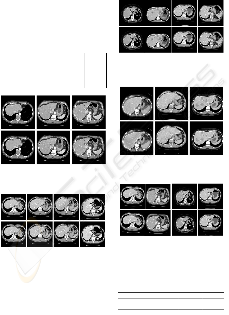
Figure 3: Samples of The proposed technique results, the
first experiment, on slices of the same patient used in the
training stage, the manual segmentation on the upper row
and the results on the bottom row.
Figure 4: Samples of The proposed technique results, the
first experiment, on slices of patients other than the one
used in the training stage, the manual segmentation on the
upper row and the results on the bottom row.
In addition, the proposed technique did not produce
any overlap with the undesired objects and it is not
affected by the abnormal tissues as noticed in
Figure5 and Figure6.
Figure 5: Samples of The proposed technique results, the
second experiment, on test slices extracted from the
patients used in the training stage, the manual
segmentation on the upper row and the results on the
bottom row.
Figure 6: Samples of The proposed technique results, the
second experiment, on novel test slices extracted from the
test patients, the manual segmentation on the upper row
and the results on the bottom row.
Figure 7: Samples of genetic algorithm-based
segmentation technique results, (a) the first experiment,
(b) the second experiment, the manual segmentation on
the upper row and the results on the bottom row.
Table 4: Goodness of fitness, G, of the final segmentation
results obtained using the different techniques (second
experiment).
The segmentation technique
Training
patients
test slices
The proposed technique
0.94 0.92
Active contour without edges
0.72 0.74
Wavelet packet decomposition
0.50 0.48
GA-based technique
0.85 0.79
ICAART 2010 - 2nd International Conference on Agents and Artificial Intelligence
296

5 CONCLUSIONS AND FUTURE
WORK
In this work, the high level features extracted using
the over-complete wavelet decomposition allows the
technique to accurately discriminate the desired
tissue. Also, the incorporation of prior shape model
in the form of mean shape and shape variability as
described in Section2 increases the ability to capture
the desired object variations without overlapping
with the other objects.
Furthermore, the direct optimization using the
particle swarm optimization algorithm eliminates the
necessitate of deriving gradient of energy or solving
complicated differential equations and it does not
need level set re-initialization. Moreover, the PSO
algorithm can efficiently explore the search space to
converge to the desired object and its parameters can
be easily adapted for any object. So the proposed
PSO segmentation technique is very suitable for the
segmentation of abdominal CT scans and it shows
promised results. Additionally, the comparison with
other techniques shows the superiority of the
proposed technique.
REFERENCES
Bankman I. (2000), hand book of medical imaging,
processing and analysis, academic press.
Chan T., Vese L. (2001), Active Contour Without edges,
IEEE transactions on image processing, 10(2), 266-
277.
Chi Z., and Wang P. (2000), A New Method of Color
Image Segmentation Based on Intensity and Hue
Clustering, 15th International Conference on Pattern
Recognition (ICPR'00), 3, 3617.
Clerc M. (2006), Particle Swarm Optimization, ISTE Ltd.
Dzung L., Chenyang X., and Jerry L. (2000), Current
Methods in Medical Image segmentation, Annual
Review of Biomedical Engineering, 2(1), 315-337.
Franc V., and Hlavac V. (2004), Statistical Pattern
Recognition Toolbox for Matlab, Prague, Czech:
Center for Machine Perception, Czech Technical
University.
Ghosh P., and Michell M. (2006), Segmentation of
Medical Images Using Genetic Algorithm,
Proceedings of the 8
th
annual conference on Genetic
and evolutionary computation, 1171-1178.
Hassan R., Cohanim B., Weck O. (2005) , A comparison of
particle swarm optimization and the genetic
algorithm, 46
th
AIAA/ASME/ASCE/AHS/ASC
Structures, Structural Dynamics, and Materials
Conference,1-13.
Kass M., Witkin A., and Terzopoulos D. (1988), Snakes:
Active Contour Models, International Journal of
computer vision, 1(4), 321-331.
Kennedy J., and Eberhart R. (1995), Particle Swarm
Optimization, Proceedings of the IEEE international
conferences on neural networks IV, 1942-1948.
Li Y., Zhang Y., Jiang X., and et al. (2005), Segmentation
of Images Using Wavelet Packet Based Feature Set
and Clustering Algorithm, International Journal of
Information Technology”, 11(7), 112-121.
McInerney T., and Terzopoulos D. (1996), Deformable
models in medical image analysis: a survey, Medical
image analysis, 1(2), 91-108.
Osher S., and Fedkiw R. (2003), Level Set Methods and
Dynamic Implicit Surfaces, Springer-Verlag, New
York .
Pan Z., and Lu J. (2007), A Bayes-Based Region-Growing
Algorithm for Medical Image Segmentation,
Computing in Science and Engineering, 9(4)32-38.
Pohle R., and Toennies K. (2001), Segmentation of
medical images is using adaptive region growing,
SPIE Medical Imaging, 4322, 1337–1346.
Poli R., Kennedy J, and Blackwell T. (2007), Particle
Swarm Optimization: An Overview, Springer Journal
of Swarm Intelligence, 1, 33-57.
Tasi A., Yezzi A., Wells W., and et al. (2003), “A Shape-
Based Approach to the Segmentation of Medical
Imagery Using Level Sets, IEEE transaction on
medical imaging, 22(2), 137-154.
Wang Q., and Feng D. (2005), A Novel Texture Descriptor
Using Over-Complete Wavelet Transform and Its
Fractal Signature, Lecture Notes in Computer
Science, 3568, 476-486.
SHAPE PRIOR SEGMENTATION OF MEDICAL IMAGES USING PARTICLE SWARM OPTIMIZATION
297
