PROTEINS POCKETS ANALYSIS AND DESCRIPTION

Virginio Cantoni, Riccardo Gatti and Luca Lombardi

University of Pavia, Dept. of Computer Engineering and System Science, Via Ferrata 1, Pavia, Italy

Keywords:

Protein-ligand docking, Curvature analysis, Concavity tree, Travel depth, Pocket mouth area and perimeter.

Abstract:

The development of computational techniques to guide the experimental processes is an important step for the

determination of the protein functions.

The purpose of the activity here described is the characterization of the active sites in protein surfaces and their

quantitative representation. A few pocket parameters like volume, travel depth, mouth area and perimeter,

amplitude parameters, interfacial area ratio, summit density and mean summit curvature are hierarchically

accessible through a concavity tree that topologically represents the entire protein molecule.

This structural representation is particularly useful for the evaluation of binding pockets, the comparison of

the morphological similarity and the identiﬁcation of potential ligand docking.

1 INTRODUCTION

When a novel experimentally determined protein is

discovered, bioinformatics tools are used to screen

the datasets of proteins with known functionalities,

searching for candidate binding sites for the 3D struc-

ture of the new protein. Speciﬁcally, if a region in

the surface of the novel protein has similarities to the

binding site of a known protein the interactions of the

latter are expected candidates in order to discover the

unknown functionalities of the former protein.

The analysis of the binding sites of proteins and

their detection, have been developed on the basis of

different protein representations and matching strate-

gies.

CAST (Liang et al., 1998) and CASTp

(Binkowski et al., 2003) automatically locate

and compute pockets volume and mouth opening area

and circumference of pockets. The algorithm applies

3D computational geometry: a triangulation of the

protein’s surface atoms (which covers a conglomerate

of 3D tetrahedra) is analyzed through convex hull,

alpha shapes and discrete ﬂow theory. A tetrahedron

having at least a triangle that cross the void region is

designated as ’empty tetrahedraon’. Empty tetrahedra

sharing a common triangle are grouped so ’ﬂowing’

towards neighboring larger tetrahedra which act as

sink. A pocket, which is a potential binding site, is

then obtained as collection of empty tetrahedra.

PASS (Brady and Stouten, 2000) is a purely ge-

ometrical method composed of several steps. First,

the protein surface is completely covered by probe

spheres. Second, each probe is associated with a

“burial” value, which corresponds to the number of

atoms contained within a sphere of radius 8

A. Third,

the probes with a “burial” value lower than a prede-

ﬁned threshold are eliminated. Four, these three steps

are iterated (with step one applied only to the parts of

the surface covered by the probes) until no new buried

probe are added. Fifth, a probe weight, which is de-

pendent to the number of their neighboring spheres

and the extent to which they are buried, is assigned.

Finally, a shortlist of active site points (ASPs), ranked

by the probe weight, is selected by identifying the

central probes in regions that contain many spheres

with high burial count. These ASPs represent the loci

of potential binding sites.

In POCKET (Levitt and Banaszak, 1992), the pro-

tein is mapped onto a 3D grid in which a grid point be-

longs to the protein molecule if it is within 3

Afrom

an atom coordinate. The pockets are characterized as

a set of grid points, not belonging to the protein for

which a scanning along the x, y, or z-axes presents a

protein-solvent area-protein sequence (called protein-

solvent- protein event).

LIGSITE (Huang and Schroeder, 2006) extends

POCKET by scanning also along the four cubic diag-

onals in addition to the coordinates axis (in fact, the

previous pocket’s deﬁnition produces classiﬁcations

that change with the angle between the reference sys-

tem and the protein). The grid points that present a

211

Cantoni V., Gatti R. and Lombardi L. (2010).

PROTEINS POCKETS ANALYSIS AND DESCRIPTION.

In Proceedings of the First International Conference on Bioinformatics, pages 211-216

DOI: 10.5220/0002725302110216

 SciTePress

number of protein-solvent-protein events greater than

a threshold are candidate active sites.

SURFNET-ConSurf (Glaser et al., 2006), rep-

resents the pocket surface by combining geometri-

cal features together with an evolutionary charac-

teristics based on the degree of conservation of the

amino acids involved. SURFNET-ConSurf is based

on a two-stage process. In the former stage, through

SURFNET (Laskowski, 1995) the potential binding

sites in the protein surface are identiﬁed. The clefts

are detected by placing a sphere between all pairs of

atoms such that the sphere just touches each atom,

then this sphere is progressively reduced in size up to

no further intersection with other atoms are present.

The resulting sphere is retained only if its radius is

greater than a minimum size predeﬁned. Once the

clefts have been ﬁlled by spheres they can be indi-

vidually described by geometric features (e.g. the

volume). In the latter stage, the regions of the re-

sulting clefts that are distant from highly conserved

residues, as deﬁned by the ConSurf-HSSP database

(Glaser et al., 2005), are removed, thus reshaping

the cleft volumes. The second stage is based on

two parameters: the maximum allowed distance and

the minimum conservation score cutoff. The remain-

ing clefts are candidate active sites (in particular the

largest ones).

In this paper we just introduce a feature vector and

describe in details a data structure in order to rep-

resent the pocked extracted by the various methods

to improve the analysis and to reach the needed per-

formance quality. The paper is organized as follows:

in section two a short survey of features for pockets

characterization is given; in section three a data struc-

ture to describe the protein’s pockets, based on a con-

cavity tree representation, which allows the complete

description, at different scales and abstraction levels,

supporting at each level the feature vector description

previously introduced, is presented. In section four a

practical case is described. The last section ﬁve con-

tains the conclusion and the near future subsequent

activity.

2 FEATURES FOR POCKET

DESCRIPTION

The goal of this paper is the characterization of each

pocket, which is extracted by segmenting the protein

surface, through morphological and topological quan-

titative descriptors. These features are enriched with

local biochemical features (types of residues and their

characteristics) to detect and specialize the active sites

of a protein.

We are considering now a second step of the pro-

cess of active sites identiﬁcation, that is, we start

knowing the segmentation of the protein surface in a

number of pockets and tunnels. In particular, we will

refer to the method given in (Cantoni et al., 2009c) but

the technique described in the sequel is not limited to

this particular solution.

2.1 Preliminary Statements

In the discrete space the protein is deﬁned in a 3D

grid (CG) of dimension L x M x N voxels. Note

that the grid is extended one voxel beyond the min-

imum and maximum coordinate of the SES (Solvent-

Excluded Surface, also known as the molecular sur-

face or Connolly surface, generated by the envelope

of a rolling sphere over the van der Waals atoms sur-

face

) in each orthogonal direction, in this way both

SES and Convex Hull (CH) borders are inside the CG

border. The voxel resolution adopted is 0.25

A, so as

to be small enough to ensure that, with the used radii

in biomolecules atoms

, any concave depression or

convex protrusion is represented by at least one voxel.

The CH of a molecule is the smallest convex poly-

hedron that contains the molecule points. In R

the

CH is constituted by a set of facets, that are trian-

gles, and a set of ridges (boundary elements) that

are edges. A practical O(n log n) algorithm for gen-

eral dimensions CH computing, is Quickhull (Barber

and Dobkin, 1996), that uses less space and executes

faster than most of the others algorithms. Let us call

R the region between the CH and the SES (the con-

cavity volume (Borgefors and Sanniti Di Baja, 1996)),

that is:

R = CH ∩ SES (1)

and Re the connected component of R adjacent to the

CH border; that is Re and R differ for the cavities

C: the volumes completely enclosed in the macro-

molecule M:

C = CH − Re − M (2)

The region Re has been partitioned into a set of dis-

joint segments P

SES

= {P

, . . . , P

}, where N

is the number of pockets and tunnels. The partition

must satisfy the following condition:

∩ P

= ∅, i 6= j (3)

∪ · · · ∪ P

= R

(4)

The radius of the solvent sphere is usally set to the ap-

proximate radius of a water molecule.

The smallest used atom is oxygen having a Van der

Walls radius of 1.4

BIOINFORMATICS 2010 - International Conference on Bioinformatics

212

Our goal is to deﬁne a feature vector to represent, in

a discriminant way to facilitate processing and statis-

tical analysis, each pocket of P

SES

. Many vector’s pa-

rameters need a reference plane that we have identi-

ﬁed with the one to which it belongs the largest CH’s

triangle involved in the pocket.

2.2 Basic Features

The problem of deﬁning an optimal set for feature

selection is complicated because, besides building

robust models, it is also important simplifying the

amount of resources required to describe the data

accurately, without ambiguity, in a very large set

of redundant and relevant information. The expert

can help, but can usually construct only a set of

application-dependent features.

An extended set of general features that can be,

in peculiar cases, partitioned in well-organized pro-

ﬁcient subsets, is the following: i) Pocket Volume

(Laskowski et al., 1996), ii) Surface to Volume Ra-

tio, iii) Skewness and Kurtosis of Height Distribu-

tion (Blunt and Jiang, 2003), iv) Mouth Aperture (in

details we consider area, perimeter and the perime-

ter to area ratio), v) Travel Depth (Coleman and

Sharp, 2006) (Giard et al., 2008), vi) Top Peaks and

Valleys, vii) Summit Density, Mean Summit Curva-

tures (both the average of the principal curvatures of

peaks and valleys (Coleman et al., 2005), (Cantoni

et al., 2009a)), viii) Interfacial Area Ratio, and ix)

Residue Conservation (Glaser et al., 2006) (the con-

servation score for each residue in a given protein can

be obtained from the ConSurf-HSSP database (Glaser

et al., 2005)).

3 THE DATA STRUCTURE

One of the most successful approaches for shape anal-

ysis and description is the structural one. We think

that this is particularly fruitful in proteomics in which

the morphology plays a fundamental role. A complex

shape, like the Re, is segmented into its component

(the pockets set), and each pocket can be subsequently

decomposed into simpler region, and the complete de-

scription is given in terms of the region’s features and

their spatial relationship. Nevertheless, pocket shapes

can be rather complex and not directly decomposable

into simpler regions. However we can re-apply the

segmentation process of the Re into the pockets. This

process can be executed recursively. In this way a se-

quence of approximations is built, and, at each stage,

exact measures of the remaining concavities, based on

the parameters described above, are given. This struc-

tural hierarchical description and analysis, guided by

the concavities (Borgefors and Sanniti Di Baja, 1992),

seems to us a very promising effective description.

The basic structure of the approach was ﬁrstly in-

troduced in (Arcelli and Sanniti Di Baja, 1978) and in

(Borgefors and Sanniti Di Baja, 1996) has been ﬁnally

called concavity tree: “components of C (Re in our

3D case) for which the internal section of the perime-

ter (surface in 3D) exceeds the external section are

structured concavities. A more sophisticated anal-

ysis of these regions is performed to extract further

features. The envelopes CH of the concavity regions

are computed using the same process as that applied

to the original pattern. Merging can occur while ﬁll-

ing meta-concavities, so the concavity regions must

be labeled and processed individually. For each con-

cavity region, its meta-concavities are identiﬁed. The

process continues until all regions are convex”.

The ﬁnal result is a hierarchical structure, the

(meta) concavity tree. At each level the concavities

can be analyzed and described on the basis of the

above feature vector - computed at each node: ob-

viously the features deﬁned for concavities can also

be computed for the meta-concavities.

The “concavities” (three “pockets” and one “tun-

nel”) and four second level meta-concavities of a 2D

example are shown in Figure 1. Figure 2 shows con-

cavities and meta-concavities of level two, three and

fourth for the tunnel of level one. The corresponding

concavity tree is shown in Figure 3. Note that termi-

nating nodes, i.e. regions without signiﬁcant concav-

ities, are highlight with a bordeaux contour.

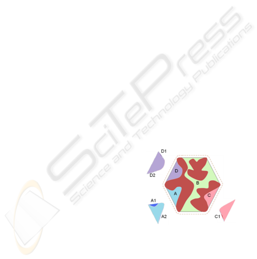
Figure 1: A 2D representation example with a tunnel and

three pockets in a section composed of three connected

components (in brown). The closed curve in black corre-

sponds to the ﬁrst level convex hull, and the border in brown

dotted-dashed line embodies the area under analysis. Part

of the second level with three meta-concavities (A, B, C)

is shown; in evidence also ﬁve third level termination-node

components (A1, A2, C1, D1, and D2).

PROTEINS POCKETS ANALYSIS AND DESCRIPTION

213

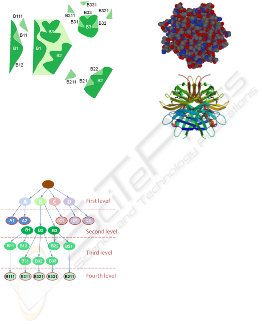
Figure 2: Continuing the 2D representation example of Fig-

ure 1, the details of the tunnel B component (light green)

are shown. The second level is composed of the three meta-

concavities (B1, B2, and B3). Each one has concavities at

the third level: B1 has a termination-node concavity (B12)

and a second component B11 which maintains a meta con-

cavity at the fourth level B111; B2 has a termination-node

concavity (B22) and a second component B21 which main-

tains a meta concavity at the fourth level B211; ﬁnally, B3

has three node concavities (B31, B32, B33) each one main-

taining a meta-concavity node-component B311, B321 and

B331 respectively, at the fourth level.

Figure 3: Representation of the concavity tree for the 2D

section of Figures 1 and 2. Note that each node contains the

information of the feature vector previously presented.

4 EXAMPLE OF A PRACTICAL

REPRESENTATION

A practical example of our hierarchical representa-

tion is given in ﬁgure 4 referring to the Apostrepta-

Figure 4: On the top the ’space ﬁlling’ representation of

1MK5. The colours follow the standard CPK scheme. On

the bottom the correspondent secondary structure represen-

tation.

vidin Wildtype Core-Streptavidin with Biotin struc-

ture (1MK5 in PDB).

As mentioned above, the analysis is accomplished

with a resolution of 0.25

A, which entails a van der

Waals radius of more than ﬁve voxels to the small-

est represented atoms. The representation is related

to the SES obtained from the quoted surface, after the

execution of a closure operator, using a sphere with

radius of 1.4

A, approximately 6 voxels, (correspond-

ing to the conventional size of a water molecule) as

structural element (see ﬁgure 5).

The segmentation of concavities and meta-

concavities is computed with the technique given in

(Cantoni et al., 2009b), where the two parameters that

characterize the execution, the minimum passage sec-

tion θ

and the maximum mouth aperture θ

have

been ﬁxed to 200 voxels (which for a circle corre-

sponds to a radius of about 8 voxels) and 2000 voxels

(which for a circle corresponds to a radius of about 25

voxels).

Figure 6 represents the complete concavity tree for

the 4 main pockets and tunnels.The molecule is rep-

resented inside its own convex hull which is drawn

completely on the backside and only through its edges

in the front side.

This process is conducted on the basis of other

two thresholds: θ

represents the minimum concav-

BIOINFORMATICS 2010 - International Conference on Bioinformatics

214

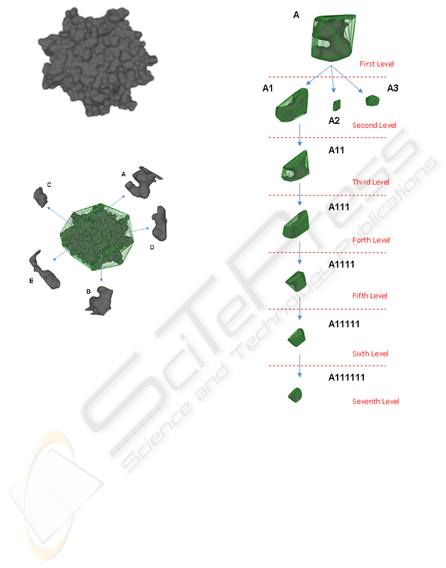
Figure 5: Solvent Excluded Surface of 1MK5 achieved

from the van der Waals surface with a sequence of dilation-

erosion operators.

Figure 6: First level of the concavity tree of the Apostrepta-

vidin Wildtype Core-Streptavidin with Biotin structure. The

representation is limited to the ﬁrst ﬁve tunnels or pockets,

ranked on the basis of the travel depth.

ity travel depth and θ

represents the minimum open

mouth at the distance θ

. These two parameters, in

the current execution, has been set to 2 voxels and 4

voxels respectively.

Figure 7 presents the sub-tree corresponding to the

largest tunnel/pocket. Following the hierarchical rep-

resentation, the volume of the components, descend-

ing the tree are more and more reduced (in fact, this

path corresponds to a multiscale process).

Note that, each node is described quantitatively

through the geometrical, topological and biochemical

parameters of the features vector described above. Fi-

nally, it is worth to point out that, as it has been shown

in (Laskowski et al., 1996) for the enzymes, the active

site is commonly found in the largest cleft.

5 CONCLUSIONS

As morphology is important for protein recognition

and function, the development of shape representa-

Figure 7: Complete hierarchical representation of the sub-

tree of the main pocket of the 1MK5, spanning six levels.

tion and analysis techniques is important in structure-

based drug development and design.

The identiﬁcation and the representation of pro-

tein cavities is a basic step for the study of sites of

activity in proteins. In this paper we presented a gen-

eral framework to evaluate geometric and topologic

parameters to represent size and form of the pock-

ets and biochemical feature, in a hierarchical multi-

level data-structure. This description is suited for the

implementation of automatic procedures for the anal-

ysis, the prediction and the comparison of potential

binding sites.

What is important now is to proceed to a statisti-

PROTEINS POCKETS ANALYSIS AND DESCRIPTION

215

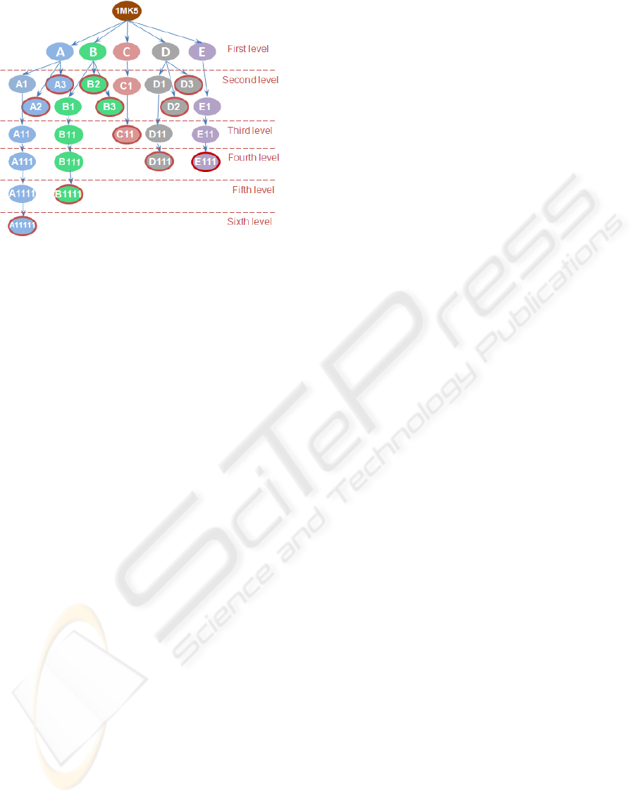
Figure 8: Complete concavity tree of the ﬁve main pockets

of the 1MK5.

cal selection of a subset of relevant features for build-

ing robust models. The exclusion of redundant fea-

tures, by reducing the dimension of the parameter

space, improves the time performance and facilitates

fast searching, processing and statistical analysis.

REFERENCES

Arcelli, C. and Sanniti Di Baja, G. (1978). Polygonal cov-

ering and concavity tree of binary digital pictures. In

Proceeding International Conference MECO 78, page

292297.

Barber, C. B. and Dobkin, D. P. (1996). The quickhull algo-

rithm for convex hulls. ACM Transactions on Mathe-

matical Software, 22:469–483.

Binkowski, A. T., Naghibzadeh, S., and Liang, J. (2003).

Castp: Computed atlas of surface topography of pro-

teins. Nucl. Acids Res., 31(13):3352–3355.

Blunt, L. and Jiang, X. (2003). Advanced Techniques for As-

sessment Surface Topography (1st edn.). Penton Press,

London.

Borgefors, G. and Sanniti Di Baja, G. (1992). Methods for

hierarchical analysis of concavities. In Proceedings of

the Conference on Pattern Recognition (ICPR), vol-

ume 3, pages 171–175.

Borgefors, G. and Sanniti Di Baja, G. (1996). Analyzing

non convex 2d and 3d patterns. Computer Vision and

Image Understanding, 63(1):145–157.

Brady, G. P. and Stouten, P. F. (2000). Fast prediction and

visualization of protein binding pockets with pass. J

Comput Aided Mol Des, 14(4):383–401.

Cantoni, V., Gatti, R., and Lombardi, L. (2009a). Ap-

proaches for protein surface curvature analysis. In

ICIAP 2009, in press.

Cantoni, V., Gatti, R., and Lombardi, L. (2009b). Proteins

pockets quantitative description. In DIS-UNIPV inter-

nal report.

Cantoni, V., Gatti, R., and Lombardi, L. (2009c). Segmen-

tation of ses for protein structure analysis. In BIOIN-

FORMATICS 2010, submitted to.

Coleman, R. G., Burr, M. A., Souvaine, D. L., and Cheng,

A. C. (2005). An intuitive approach to measuring pro-

tein surface curvature. Proteins, 61(4):1068–1074.

Coleman, R. G. and Sharp, K. A. (2006). Travel depth, a

new shape descriptor for macromolecules: application

to ligand binding. J Mol Biol, 362(3):441–458.

Giard, J., Patrice, R. A., and Macq, B. (2008). Fast and

accurate travel depth estimation for protein active site

prediction. SPIE Electronic Imaging, San Jose 2008,

pages 0Q–10Q.

Glaser, F., Morris, R. J., Najmanovich, R. J., Laskowski,

R. A., and Thornton, J. M. (2006). A method for lo-

calizing ligand binding pockets in protein structures.

Proteins, 62(2):479–488.

Glaser, F., Rosenberg, Y., Kessel, A., Pupko, T., and Ben-

Tal, N. (2005). The consurf-hssp database: the map-

ping of evolutionary conservation among homologs

onto pdb structures. Proteins, 58(3):610–617.

Huang, B. and Schroeder, M. (2006). Ligsitecsc: predict-

ing ligand binding sites using the connolly surface

and degree of conservation. BMC Structural Biology,

6(1):19+.

Laskowski, R. A. (1995). Surfnet: a program for visual-

izing molecular surfaces, cavities, and intermolecular

interactions. J Mol Graph, 13(5).

Laskowski, R. A., Luscombe, N. M., Swindells, M. B., and

Thornton, J. M. (1996). Protein clefts in molecular

recognition and function. Protein Sci, 5(12):2438–

2452.

Levitt, D. G. and Banaszak, L. J. (1992). Pocket: a com-

puter graphics method for identifying and displaying

protein cavities and their surrounding amino acids. J

Mol Graph, 10(4):229–234.

Liang, J., Edelsbrunner, H., and Woodward, C. (1998).

Anatomy of protein pockets and cavities: measure-

ment of binding site geometry and implications for

ligand design. Protein Sci, 7(9):1884–1897.

BIOINFORMATICS 2010 - International Conference on Bioinformatics

216