
MODEL-FREE LEARNING FROM DEMONSTRATION
Erik A. Billing, Thomas Hellstr¨om and Lars-Erik Janlert
Department of Computing Science, Ume˚a University, Ume˚a, Sweden
Keywords:
Learning from demonstration, Prediction, Robot imitation, Motor control, Model-free learning.
Abstract:
A novel robot learning algorithm called Predictive Sequence Learning (PSL) is presented and evaluated. PSL
is a model-free prediction algorithm inspired by the dynamic temporal difference algorithm S-Learning. While
S-Learning has previously been applied as a reinforcement learning algorithm for robots, PSL is here applied
to a Learning from Demonstration problem. The proposed algorithm is evaluated on four tasks using a Khepera
II robot. PSL builds a model from demonstrated data which is used to repeat the demonstrated behavior. After
training, PSL can control the robot by continually predicting the next action, based on the sequence of passed
sensor and motor events. PSL was able to successfully learn and repeat the first three (elementary) tasks, but
it was unable to successfully repeat the fourth (composed) behavior. The results indicate that PSL is suitable
for learning problems up to a certain complexity, while higher level coordination is required for learning more
complex behaviors.
1 INTRODUCTION
Recent years have witnessed an increased interest
in computational mechanisms that will allow robots
to Learn from Demonstrations (LFD). With this ap-
proach, also referred to as Imitation Learning, the
robot learns a behavior from a set of good examples,
demonstrations. The field has identified a number of
key problems, commonly formulated as what to imi-
tate, how to imitate, when to imitate and who to im-
itate (Billard et al., 2008). In the present work, we
focus on the first question, referring to which aspects
of the demonstration should be learned and repeated.
Inspiration is taken from several functional mod-
els of the brain and prediction is exploited as a way
to learn state definitions. A novel learning algo-
rithm, called Predictive Sequence Learning (PSL), is
here presented and evaluated. PSL is inspired by
S-Learning (Rohrer and Hulet, 2006a; Rohrer and
Hulet, 2006b), which has previously been applied to
robot learning problems as a model-free reinforce-
ment learning algorithm (Rohrer, 2009; Rohrer et al.,
2009).
The paper is organized as follows. In Section 2
a theoretical background and biological motivation is
given. Section 3 gives a detailed description of the
proposed algorithm. Section 4 describes the exper-
imental setup and results for evaluation of the algo-
rithm. In Section 5, conclusions, limitations and fu-
ture work are discussed.
2 MOTIVATION
One common approach to identify what in a demon-
stration that is to be imitated is to exploit the variabil-
ity in several demonstrations of the same behavior.
Invariants among the demonstrations are seen as the
most relevant and selected as essential components of
the task (Billard et al., 2008; Delson and West, 1994).
Several methods for discovering invariants in demon-
strations can be found in the LFD literature. One
method presented by Billard and co-workers applies
a time-delayed neural network for extraction of rele-
vant features from a manipulation task (Billard et al.,
2003; Billard and Mataric, 2001). A more recent ap-
proach uses demonstrations to impose constraints in a
dynamical system, e.g. (Calinon et al., 2007; Guenter
et al., 2007).
While this is a suitable method for many types
of tasks, there are also applications where it is less
obvious which aspects of a behavior should be in-
variant, or if the relevant aspects of that behavior is
captured by the invariants. Since there is no uni-
versal method to determine whether two demonstra-
tions should be seen as manifestations of the same
behavior or two different behaviors (Billing and Hell-
strm, 2008b), it is in most LFD applications up to
62
A. Billing E., Hellström T. and Janlert L. (2010).
MODEL-FREE LEARNING FROM DEMONSTRATION.
In Proceedings of the 2nd International Conference on Agents and Artificial Intelligence - Agents, pages 62-71
DOI: 10.5220/0002729500620071
Copyright
c
SciTePress

the teacher to decide. However, the teacher’s group-
ing of actions into behaviors may not be useful for
the robot. In the well known imitation framework
by Nehaniv and Dautenhahn (Nehaniv and Dauten-
hahn, 2000), it is emphasized that the success of an
imitation is observer dependent. The consequence
of observer dependence when it comes to interpret-
ing sequences of actions has been further illustrated
with Pfeifer and Scheier’s argument about the frame
of reference (Pfeifer and Scheier, 1997; Pfeifer and
Scheier, 2001), and is also reflected in Simon’s para-
ble with the ant (Simon, 1969). A longer discussion
related to these issues can be found in (Billing, 2007).
Pfeifer and Scheier promotes the use of a low
level specification (Pfeifer and Scheier, 2001), and
specifically the sensory-motor space I =U ×Y, where
U and Y denotes the action space and observation
space, respectively. Representations created directly
in I prevents the robot from having memory, which
has obvious limitations. However, systems with no
or very limited memory capabilities has still reached
great success within the robotics community through
the works by Rodney Brooks, e.g., (Brooks, 1990;
Brooks, 1991a; Brooks, 1991b; Brooks, 1986), and
the development of the reactive and behavior based
control paradigms, e.g., (Arkin, 1998). By extend-
ing the definition of I such that it captures a cer-
tain amount of temporal structure, the memory limi-
tation can be removed. Such a temporally extended
sensory-motor space is denoted history information
space I
τ
= I
0
× I
1
× I
2
× ... × I
τ
, where τ denotes the
temporal extension of I (Billing and Hellstrm, 2008b).
With a large enough τ, I
τ
can model any behavior.
However, a large τ leads to an explosion of the num-
ber of possible states, and the robot has to generalize
such that it can act even though the present state has
not appeared during training.
In the present work, we present a learning method
that is not based on finding invariants among several
demonstrations of, what the teacher understands to
be “the same behavior”. Taking inspiration from re-
cent models of the brain where prediction plays a cen-
tral role, e.g. (Friston, 2003; George, 2008; Haruno
et al., 2001; Lee and Mumford, 2003), we approach
the question of what to imitate by the use of predic-
tion.
2.1 Functional Models of Cortex
During the last two decades a growing body of re-
search has proposed computational models that aim
to capture different aspects of human brain function,
specifically the cortex. This research includes models
of perception, e.g., Riesenhuber and Poggio’s hierar-
chical model (Riesenhuber and Poggio, 1999) which
has inspired several more recent perceptual models
(George, 2008; Lee and Mumford, 2003; Poggio and
Bizzi, 2004), models of motor control (Haruno et al.,
2003; Rohrer and Hulet, 2006a; Wolpert and Ghahra-
mani, 2000; Wolpert and Flanagan, 2001; Wolpert,
2003) and learning (Friston, 2003). In 2004, this
field reached a larger audience with the release of
Jeff Hawkins’s book On Intelligence (Hawkins and
Blakeslee, 2002). With the ambition to present a uni-
fied theory of the brain, the book describes cortex
as a hierarchical memory system and promotes the
idea of a common cortical algorithm. Hawkins’s the-
ory of cortical function, referred to as the Memory-
Prediction framework, describes the brain as a predic-
tion system. Intelligence is, in this view, more about
applying memories in order to predict the future, than
it is about computing a response to a stimulus.
A core issue related to the idea of a common cor-
tical algorithm is what sort of bias the brain uses. One
answer is that the body has a large number of reward
systems. These systems are activated when we eat,
laugh or make love, activities that through evolution
have proved to be important for survival. However,
these reward systems are not enough. The brain also
needs to store the knowledge of how to activate these
reward systems.
In this context, prediction appears to be critical for
learning. The ability to predict the future allows the
agent to foresee the consequences of its actions and
in the long term how to reach a certain goal. How-
ever, prediction also plays an even more fundamental
role by providing information about how well a cer-
tain model of the world correlates with reality.
This argument is supported not only by Hawkins’s
work, but by a large body of research investigating
the computational aspects of the brain. It has been
proposed that the central nervous system (CNS) sim-
ulates aspects of the sensorimotor loop (Jordan and
Rumelhart, 1992; Kawato et al., 1987; Miall and
Wolpert, 1996; Wolpert and Flanagan, 2001). This in-
volves a modular view of the CNS, where each mod-
ule implements one forward model and one inverse
model. The forward model predicts the sensory con-
sequences of a motor command, while the inverse
model calculates the motor command that, in the cur-
rent state, leads to the goal (Wolpert, 2003). Each
module works under a certain context or bias, i.e., as-
sumptions about the world which are necessary for the
module’s actions to be successful. One purpose of the
forward model is to create an estimate of how well the
present situation corresponds to these assumptions. If
the prediction error is low the situation is familiar.
However, if the prediction error is high, the situation
MODEL-FREE LEARNING FROM DEMONSTRATION
63

does not correspond to the module’s context and ac-
tions produced by the inverse model may be inappro-
priate.
These findings have inspired recent research on
robot perception and control. One example is the
rehearse, predict, observe, reinforce decomposition
proposed by Demiris and others (Demiris and Hayes,
2002; Demiris and Simmons, 2006; Schaal et al.,
2003) which adapts the view of perception and action
as two aspects of a single process. Hierarchical rep-
resentations following this decomposition have also
been tested in an LFD setting (Demiris and Johnson,
2003) where the robot successfully learns sequences
of actions from observation. The present work should
be seen as a further investigation of these theories ap-
plied to robots, with focus to learning with minimal
bias.
2.2 Sequence Learning
The learning algorithm presented in this paper, re-
ferred to as Predictive Sequence Learning (PSL), is
inspired by S-Learning, a dynamic temporal differ-
ence (TD) algorithm presented by Rohrer and Hulet,
(Rohrer and Hulet, 2006a; Rohrer and Hulet, 2006b).
S-Learning builds sequences of passed events which
may be used to predict future events, and in contrast
to most other TD algorithms it can base its predictions
on many previous states.
S-Learning can be seen as a variable order Markov
model (VMM) and we have observed that it is very
similar to the well known compression algorithm
LZ78 (Ziv and Lempel, 1978). This coincidence is
not that surprising considering the close relationship
between loss-less compression and prediction (Be-
gleiter and Yona, 2004). In principle, any lossless
compression algorithm could be used for prediction,
and vice versa (Feder and Merhav, 1994).
S-Learning was originally developed to capture
the discrete episodic properties observed in many
types of human motor behavior (Rohrer, 2007). It
takes inspiration from the Hierarchical Temporal
Memory algorithm (George and Hawkins, 2005), with
focus on introducing as few assumptions into learning
as possible. More recently, it has been applied as a
model-free reinforcement learning algorithm for both
simulated and physical robots (Rohrer, 2009; Rohrer
et al., 2009). We have also evaluated S-Learning as an
algorithm for behavior recognition (Billing and Hell-
strm, 2008a). However, to our knowledge it has never
been used as a control algorithm for LFD.
The model-free design of S-Learning, together
with its focus on sequential data and its connections
to human motor control makes S-Learning very inter-
esting for further investigation as a method for robot
learning. With the ambition to increase the focus on
prediction, and propose a model that automatically
can detect when it is consistent with the world, PSL
was designed.
3 PREDICTIVE SEQUENCE
LEARNING
PSL is trained on an event sequence η =
(e
1
,e
2
,. .. ,e
t
), where each event e is a member
of an alphabet
∑
. η is defined up to the current time t
from where the next event e
t+1
is to be predicted.
PSL stores its knowledge as a set of hypotheses,
known as a hypothesis library H. A hypothesis h ∈ H
expresses a dependence between an event sequence
X = (e
t− n
,e
t− n+1
,. .. ,e
t
) and a target event I = e
t+1
:
h : X ⇒ I (1)
X
h
is referred to as the body of h and I
h
denotes the
head. Each h is associated with a confidence c reflect-
ing the conditional probability P(I|X). For a given
η, c is defined as c(X ⇒ I) = s(X,I) /s(X), where
the support s(X) describes the proportion of transac-
tions in η that contains X and (X, I) denotes the con-
catenation of X, and I. A transaction is defined as a
sub-sequence of the same size as X. The length of h,
denoted |h|, is defined as the number of elements in
X
h
. Hypotheses are also referred to as states, since a
hypothesis of length |h| corresponds to VMM state of
order |h|.
3.1 Detailed Description of PSL
Let the library H be an empty set of hypotheses. Dur-
ing learning, described in Algorithm 1, PSL tries to
predict the future event e
t+1
, based on the observed
event sequence η. If it fails to predict the future state,
a new hypothesis h
new
is created and added to H. h
new
is one element longer than the longest matching hy-
pothesis previously existing in H. In this way, PSL
learns only when it fails to predict.
For example, consider the event sequence η =
ABCCABCCA. Let t = 1. PSL will search for a
hypothesis with a body matching A. Initially H is
empty and consequently PSL will create a new hy-
pothesis (A) ⇒ B which is added to H. The same
procedure will be executed at t = 2 and t = 3 so that
H = {(A) ⇒ B;(B) ⇒ C;(C) ⇒ C}. At t = 4, PSL
will find a matching hypothesis h
max
: (C) ⇒ C pro-
ducing the wrong prediction C. Consequently, a new
hypothesis (C) ⇒ A is added to H. The predictions at
ICAART 2010 - 2nd International Conference on Agents and Artificial Intelligence
64

t = 5 and t = 6 will be successful while h : (C) ⇒ A
will be selected at t = 7 and produce the wrong pre-
diction. As a consequence, PSL will create a new
hypothesis h
new
: (B,C) ⇒ C. Source code from the
implementation used in the present work is available
online (Billing, 2009).
Algorithm 1. Predictive Sequence Learning (PSL).
Given an event sequence η = (e
1
,e
2
,. .. ,e
n
)
1. Let the current time t = 1 and the library H =
/
0
2. Let M ⊆ H be all hypotheses h with X
h
=
e
t− |h|+1
,e
t− |h|+2
,. .. ,e
t
3. If M =
/
0
(a) Create a new hypothesis h
new
: (e
t
) ⇒ e
t+1
(b) Add h
new
to H
(c) Continue from 6
4. Let h
max
be the longest hypothesis h ∈ M. If sev-
eral hypotheses with the same length exist, select
the one with highest confidence c.
5. If e
t+1
6= I
h
max
(a) Let h
correct
∈ H be the longest hypothesis h ∈ M
with I
h
= e
t+1
(b) If no such hypothesis exists in H, create a new
hypothesis h
new
: (e
t
) ⇒ e
t+1
(c) Otherwise, create a new hypothesis h
new
:
e
t− |h
correct
|
,e
t− |h
correct
|+1
,e
t− |h
correct
|+2
,. .. ,e
t
⇒
e
t+1
(d) Add h
new
to H
6. Update the confidence for h
max
and h
correct
as de-
scribed in Section 3
7. Set t = t + 1
8. If t < n, then continue from 2.
Algorithm 2. Making predictions using PSL.
Given an event sequence η = (e
1
,e
2
,. .. ,e
t
)
1. Let M ⊆ H be all hypotheses h with X
h
=
e
t− |h|+1
,e
t− |h|+2
,. .. ,e
t
2. Let h
max
be the longest hypothesis h ∈ M. If sev-
eral hypothesis with the same length exists, select
the one with highest confidence c.
3. Return the prediction e
′
t+1
= I(h
max
)
3.2 Making Predictions
After, or during, learning, PSL can be used to make
predictions based on the sequence of passed events
η = (e
1
,e
2
,. .. ,e
t
). Since PSL continuously makes
predictions during learning, this procedure is very
similar to the learning algorithm (Algorithm 1). The
prediction procedure is described in Algorithm 2.
For prediction of a suite of future events, e
′
t+1
can
be added to η to create η
′
. Then repeat the procedure
described in Algorithm 2 using η
′
as event history.
3.3 Differences and Similarities between
PSL and S-Learning
Like PSL, S-Learning is trained on an event sequence
η. However, S-Learning does not produce hypothe-
ses. Instead, knowledge is represented as Sequences
φ, stored in a sequence library κ (Rohrer and Hulet,
2006b). φ does not describe a relation between a body
and a head, like hypotheses do. Instead, φ describes
a plain sequence of elements e ∈ η. During learning,
sequences are “grown” each time a matching pattern
for that sequence appears in the training data. Com-
mon patterns in η produce long sequences in κ. When
S-Learning is used to predict the next event, the be-
ginning of each φ ∈ κ is matched to the end of η. The
sequence producing the longest match is selected as a
winner, and the end of the winning sequence is used
to predict future events.
One problem with this approach, observed during
our previous work with S-Learning (Billing and Hell-
strm, 2008a), is that new, longer sequences, are cre-
ated even though the existing sequence already has
Markov property, meaning that it can predict the next
element optimally. To prevent the model from getting
unreasonably large, S-Learning implements a max-
imum sequence length m. As a result, κ becomes
unnecessarily large, even when m is relatively low.
More importantly, by setting the maximum sequence
length m, a task-dependent modeling parameter is
introduced, which may limit S-Learning’s ability to
model η.
PSL was designed to alleviate the problems with
S-Learning. Since PSL learns only when it fails to
predict, it is less prune to be overtrained and can em-
ploy an unlimited maximum sequence length without
exploding the library size.
4 EVALUATION
The PSL algorithm was tested on a Khepera II minia-
ture robot (K-Team, 2007). In the first evaluation
(Section 4.1), the performance of PSL on a play-
ful LFD task is demonstrated. During both experi-
ments, the robot is given limited sensing abilities us-
ing only its eight infrared proximity sensors mounted
around its sides. In a second experiment (Section 4.2),
MODEL-FREE LEARNING FROM DEMONSTRATION
65

the prediction performance during training of PSL is
compared to the performance of S-Learning, using
recorded sensor and motor data from the robot.
One important issue, promoted both by Rohrer
with colleagues (Rohrer et al., 2009; Rohrer, 2009)
and ourselves (Billing and Hellstrm, 2008b), is the
ability to learn even with limited prior knowledge of
what is to be learned. Prior knowledge is informa-
tion intentionally introduced into the system to sup-
port learning, often referred to as ontological bias or
design bias (Billing and Hellstrm, 2008b). Examples
of common design biases are pre-defined state spec-
ifications, pre-processing of sensor data, the size of
a neural network, the length of a temporal window
or other “tweaking” parameters. While design biases
help in learning, they also limit the range of behaviors
a robot can learn. Furthermore, a system implement-
ing large amounts of design bias will to a larger extent
base its decisions not on its own experience, but on
knowledge of the programmer designing the learning
algorithm, making it hard to determine what the sys-
tem has actually learned.
In addition to design bias, there are many limita-
tions and constraints introduced by other means, e.g.,
by the size and shape of the robot including its sensing
and action capabilities, structure of the environment
and performance limitations of the computer used.
These kinds of limitations are referred to as prag-
matical bias. We generally try to limit the amount
of ontological bias, while pragmatical bias should be
exploited by the learning algorithm to find valuable
patterns.
In the present experiments, the robot has no pre-
vious knowledge about its surroundings or itself. The
only obvious design bias is the thresholding of prox-
imity sensors into three levels, far, medium and close,
corresponding to distances of a few centimeters. This
thresholding was introduced to decrease the size of
the observation space Y, limiting the amount of train-
ing required. An observation y ∈ Y is defined as the
combination of the eight proximity sensors, produc-
ing a total of 3
8
possible observations.
An action u ∈ U is defined as the combination of
the speed commands sent to the two motors. The
Khepera II robot has 256 possible speeds for each
wheel, producing an action space U of 256
2
possible
actions. However, only a small fraction of these were
used during demonstration.
The event sequence is built up by alternating sen-
sor and action events, η = (u
1
,y
1
,u
2
,y
2
.. ., u
k
,y
k
). k
is here used to denote the current stage, rather than
the current position in η denoted by t. Even though
events is categorized into observations and actions,
PSL makes no distinction between these two types
of events. From the perspective of the algorithm, all
events e
t
∈
∑
are discrete entities with no predefined
relations, where
∑
= Y ∪U.
In each stage k, PSL is used to predict the next
event, given η. Since the last element of η is an ob-
servation, PSL will predict an action u
k
∈ U, leading
to the observation y
k
∈ Y. u
k
and y
k
are appended
to η, transforming stage k to k + 1. This alternat-
ing use of observations and actions was adopted from
S-Learning (Rohrer and Hulet, 2006a). A stage fre-
quency of 10 Hz was used, producing one observation
and one action every 0.1 seconds.
4.1 Demonstration and Repetition of
Temporally Structured Behavior
To evaluate the performance of PSL on an LFD prob-
lem, four tasks are defined and demonstrated using the
Khepera II robot. Task 1 involves the robot moving
forward in a corridor approaching an object (cylindri-
cal wood block). When the robot gets close to the
object, it should stop and wait for the human teacher
to “load” the object, i.e., place it upon the robot. After
loading, the robot turns around and goes back along
the corridor. Task 2 involves general corridor driving,
taking turns in the right way without hitting the walls
and so on. Task 3 constitutes the “unloading” proce-
dure, where the robot stops in a corner and waits for
the teacher to remove the object and place it to the
right of the robot. Then the robot turns and pushes
the cylinder straight forward for about 10 centime-
ters, backs away and turns to go for another object.
Task 4 is the combination of the three previous tasks.
The sequence of actions expected by the robot is illus-
trated in Figure 1 and the experimental setup can be
seen in Figure 2. Even though the setup was roughly
the same in all experiments, the starting positions and
exact placement of the walls varied between demon-
stration and repetition.
All tasks capture a certain amount of temporal
structure. One example is the turning after loading
the object in Task 1. Exactly the same pattern of sen-
sor and motor data will appear before, as well as after,
turning. However, two different sequences of actions
is expected. Specifically, after the teacher has taken
the cylinder to place it on the robot, only the sensors
on the robot’s sides are activated. The same sensor
pattern appears directly after the robot has completed
the 180 degree turn, before it starts to move back
along the corridor. Furthermore, the teacher does not
act instantly. After placing the object on the robot,
one or two seconds passed before the teacher issued
a turning command, making it more difficult for the
learning algorithm to find the connection between the
ICAART 2010 - 2nd International Conference on Agents and Artificial Intelligence
66
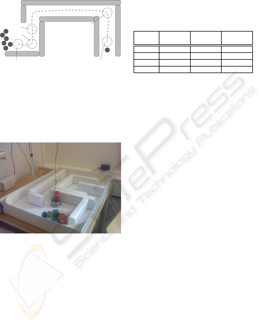
wait for loading,
then turn and go back
turn
start
unload
push object
Figure 1: Schematic overview of the composed behavior
(Task 4). Light gray rectangles mark walls, dark gray cir-
cles mark the objects and dashed circles mark a number
of key positions for the robot. The robot starts by driving
upwards in the figure, following the dashed line. until it
reaches the object at the loading position. After loading,
the robot turns around and follows the dashed line back un-
til it reaches the unload position. When the cylinder has
been unloaded (placed to the left of the robot), the robot
turns and pushes the object. Finally, it backs away from the
pile and awaits further instructions.
Figure 2: Experimental setup.
events. Even Task 2 which is often seen as a typi-
cal reactive behavior is, due to the heavy thresholding
of sensor data, temporally demanding. Even longer
temporal structures can be found in Task 3, where
the robot must push the object and remember for how
long the object is to be pushed. This distance was not
controlled in any way, making different demonstra-
tions of the same task containing slightly conflicting
data.
Results. After training, the robot was able to re-
peat Task 1, 2 and 3 successfully. For Task 1, seven
demonstrations was used for a total of about 2.6 min.
Task 2 was demonstrated for about 8.7 min and Task
3 was demonstrated nine times, in total 4.6 min. The
robot did occasional mistakes in all three tasks, reach-
Table 1: Detailed statistics on the four evaluation tasks.
Training events is the number of sensor and motor events
in demonstrated data. Lib. size is the number of hypotheses
in library after training. Avg. |h| is the average hypothesis
length after training.
Task Training
events
Lib. size Avg. |h|
Task 1 3102 4049 9.81
Task 2 10419 30517 16
Task 3 5518 8797 11
Task 4 26476 38029 15
ing situations where it had no training data. In these
situations it sometimes needed help to be able to com-
plete the task. However, the number of mistakes
clearly decreased with increased training, and mis-
takes made by the teacher during training often helped
the robot to recover from mistakes during repetition.
For Task 4, the demonstrations from all three par-
tial tasks were used, plus a single 2 min demonstra-
tion of the entire Task 4. Even after extensive train-
ing, resulting in almost 40 000 hypotheses in library,
the robot was unable to repeat the complete behavior
without frequent mistakes. Knowledge from the dif-
ferent sub-tasks was clearly interfering, causing the
robot to stop and wait for unloading when it was sup-
posed to turn, turning when it was supposed to follow
the wall and so on. Detailed results for all four tasks
can be found in Table 1.
PSL was trained until it could predict about 98%
of the demonstrated data correctly. It would be pos-
sible to train it until it reproduces all events correctly,
but this takes time and initial experiments showed
that it did not affect the imitation performance sig-
nificantly.
4.2 Comparison between S-Learning
and PSL
In Section 3.3, a number of motivations for the de-
sign of PSL were given, in relation to S-Learning.
One such motivation was the ability to learn and
increase the model size only when necessary. S-
Learning always learns and creates new sequences
for all common events, while PSL only learns when
prediction fails. However, it should be pointed out
that even though S-Learning never stops to learn un-
less an explicit limit on sequence length is introduced,
it quickly reduces the rate at which new sequences
are created in domains where it already has extensive
knowledge.
To evaluate the effect of these differences between
PSL and S-Learning, prediction performance and li-
brary size was measured during training in three test
MODEL-FREE LEARNING FROM DEMONSTRATION
67
cases. Case 1 contained a demonstration of the load-
ing procedure (Task 1) used in the LFD evaluation,
Section 4.1. During the demonstration, the procedure
was repeated seven times for a total of about 150 sec-
onds (3000 sensor and motor events). Case 2 encap-
sulated the whole composed behavior (Task 4) used
in LFD evaluation. The behavior was demonstrated
once for 120 seconds (2400 events). Case 3 consti-
tuted 200 seconds of synthetic data, describing a 0.1
Hz sinus wave discretized with a temporal resolution
of 20 Hz and an amplitude resolution of 0.1 (resulting
in 20 discrete levels). The 4000 elements long data
sequence created a clean repetitive pattern with minor
fluctuations due to sampling variations.
In addition to PSL and S-Learning, a first order
Markov model (1MM) was included in the tests. The
Markov model can obviously not learn the pattern in
any of the three test cases perfectly, since there is no
direct mapping e
t
⇒ e
t+1
for most events. Hence, The
1MM should be seen only as a base reference.
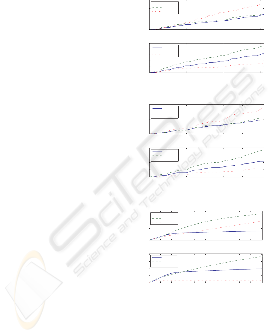
Results. Figures 3, 4 and 5 displays results from the
three test cases. The upper plot of each figure repre-
sents the accumulated error count for each of the three
learning algorithms. The lower plot shows the model
size (number of sequences in library) for PSL and S-
Learning. Since the Markov model does not have a
library, the number of edges in the Markov graph is
shown, which best corresponds to sequences or hy-
potheses in S-Learning and PSL, respectively.
5 DISCUSSION
In the present work, a novel robot learning algorithm
called Predictive Sequence Learning (PSL) is pre-
sented and evaluated in an LFD setting. PSL is both
parameter-free and model-free in the sense that no on-
tological information about the robot or conditions in
the world is pre-defined in the system. Instead, PSL
creates a state space (hypothesis library) in order to
predict the demonstrated data optimally. This state
space can thereafter be used to control the robot such
that it repeats the demonstrated behavior.
In contrast to many other LFD algorithms, PSL
does not build representations from invariants among
several demonstrations that a human teacher consid-
ers to be “the same behavior”. All knowledge, from
one or several demonstrations, is stored as hypothe-
ses in the library. PSL treats inconsistencies in these
demonstrations by generating longer hypotheses that
will allow it to make the correct predictions. In this
way, the ambiguous definition of behavior is avoided.
In the prediction performance comparison, PSL
0 50 100 150
0
500
1000
time (s)
error count
Accumulated training error
PSL
S-Learning
1MM
0 50 100 150
0
200
400
600
800
time (s)
library size
Model growth
PSL
S-Learning
1MM
Figure 3: Case 1 - Loading behavior. See text for details.
0 20 40 60 80 100 120
0
500
1000
time (s)
error count
Accumulated training error
PSL
S-Learning
1MM
0 20 40 60 80 100 120
0
200
400
600
time (s)
library size
Model growth
PSL
S-Learning
1MM
Figure 4: Case 2 - Composed behavior. See text for details.
0 20 40 60 80 100 120 140 160 180 200
0
500
1000
time (s)
error count
Accumulated training error
PSL
S-Learning
1MM
0 20 40 60 80 100 120 140 160 180 200
0
200
400
600
800
time (s)
library size
Model growth
PSL
S-Learning
1MM
Figure 5: Case 3 - Sinus wave. See text for details.
produces significantly smaller libraries than S-
Learning on all three data sets. The difference is par-
ticularly large in Case 3 (Figure 5), where the algo-
rithms learn to predict the data almost perfectly. In
this situation, S-Learning continues to create new se-
quences, while PSL does not.
In Case 3, PSL also shows the clearly fastest learn-
ing rates (least accumulated errors). The reason can
ICAART 2010 - 2nd International Conference on Agents and Artificial Intelligence
68

be found in that PSL learns on each event where it
fails to predict, while S-Learning learns based on se-
quence length. When the model grows, S-Learning
decreases its learning rate even though the perfor-
mance is still low. In contrast, the learning rate of PSL
is always proportional to performance, which can also
be seen in the plots for all three test cases (Figures 3,
4 and 5). However, even though PSL commits less ac-
cumulated errors than S-Learning in all three tests, the
performance difference in Case 1 and 2 is small and
how these results generalize to other kinds of data is
still an open question.
In the demonstration-repetition evaluation, tasks
1, 2 and 3 were repeated correctly. Even though the
robot made occasional mistakes, the imitation perfor-
mance clearly increased with more demonstrations.
However, in Task 4, which was a combination of
the three first tasks, an opposite pattern could be ob-
served. Despite the fact that PSL was still able to
predict demonstrated data almost perfectly, knowl-
edge from the three elementary tasks clearly inter-
fered. The reason for this interference is that Task
4 requires much longer temporal dynamics than any
of the elementary tasks did when learned separately.
One example of how this knowledge interference
is manifested is the turning versus unloading. When
the robot approaches the position marked as turn in
Figure 1, coming from the left and is supposed to take
a right turn, it no longer sees the right wall behind
it. Consequently, the situation looks identical to that
of unloading. When the robot is to unload, it goes
downward in Figure 1 (position unload) but instead
of turning it must wait for the cylinder to be placed to
its right side. To make the right prediction, PSL has
to base its decision on information relatively far back
in the event history. Even though PSL has no problem
to build a sufficiently large model from training data,
the large temporal window produces a combinatorial
explosion and the chance of the right patterns reap-
pearing during repetition is small. As a result, PSL
decreases the temporal window (i.e., uses shorter hy-
potheses), and the two situations become inseparable.
5.1 Conclusions and Future Work
The results shows that the proposed algorithm is fea-
sible for LFD problems up to a certain complexity.
PSL implements very few assumptions of what to be
learned and is therefore likely to be applicable to a
wide range of problems.
However, PSL also shows clear limitations when
the learning problem increases and longer temporal
dynamics is required. PSL is subject to combina-
torial explosion and the amount of required training
data increases exponentially with problem complex-
ity. In these situations, some higher-level coordina-
tion is clearly necessary. One possible solution is
to place PSL as a module in a hierarchical system.
PSL learns both to predict sensor data as a response
of action (forward model) and select actions based
on the current state (inverse model). In the present
work, PSL is viewed purely as a controller and the
forward model is consequently not considered. How-
ever, as discussed in Section 2.1, forward models can
play an important role in coordinating action. One ar-
chitecture exploring this direction is the hierarchical
model of human motor control known as HMOSAIC
(Haruno et al., 2003). It would be possible to consider
PSL as one part in a similar architecture. Exploiting
these possibilities will be part of our future work.
ACKNOWLEDGEMENTS
We would like to thank Brandon Rohrer at Sandia Na-
tional Laboratories and Christian Balkenius at Lund
University for valuable input to this work.
REFERENCES
Arkin, R. C. (1998). Behaviour-Based Robotics. MIT Press.
Begleiter, R. and Yona, G. (2004). On prediction using vari-
able order markov models. Journal of Artificial Intel-
ligence Research, 22:385–421.
Billard, A., Calinon, S., Dillmann, R., and Schaal, S.
(2008). Robot programming by demonstration. In
Siciliano, B. and Khatib, O., editors, Handbook of
Robotics. Springer.
Billard, A., Epars, Y., Cheng, G., and Schaal, S. (2003).
Discovering imitation strategies through categoriza-
tion of multi-dimensional data. In Proceedings
of IEEE/RSJ International Conference on Intelligent
Robots and Systems, volume 3, pages 2398–2403
vol.3.
Billard, A. and Mataric, M. J. (2001). Learning human arm
movements by imitation:: Evaluation of a biologically
inspired connectionist architecture. Robotics and Au-
tonomous Systems, 37(2-3):145–160.
Billing, E. A. (2007). Representing behavior - distributed
theories in a context of robotics. Technical report,
UMINF 0725, Department of Computing Science,
Ume University.
Billing, E. A. (2009). Cognition reversed.
http://www.cognitionreversed.com.
Billing, E. A. and Hellstrm, T. (2008a). Behavior recog-
nition for segmentation of demonstrated tasks. In
IEEE SMC International Conference on Distributed
Human-Machine Systems, pages 228 – 234, Athens,
Greece.
MODEL-FREE LEARNING FROM DEMONSTRATION
69

Billing, E. A. and Hellstrm, T. (2008b). Formalising learn-
ing from demonstration. Technical report, UMINF
0810, Department of Computing Science, Ume Uni-
versity.
Brooks, R. A. (1986). A robust layered control system for
a mobile robot. In IEEE Journal of Robotics and Au-
tomation RA-2, volume 1, pages 14–23.
Brooks, R. A. (1990). Elephants don’t play chess. Robotics
and Autonomous Systems, 6:3–15.
Brooks, R. A. (1991a). Intelligence without reason. Pro-
ceedings, 1991 Int. Joint Conf. on Artificial Intelli-
gence, pages 569–595.
Brooks, R. A. (1991b). New approaches to robotics. Sci-
ence, 253(13):1227–1232.
Calinon, S., Guenter, F., and Billard, A. (2007). On
learning, representing and generalizing a task in a
humanoid robot. IEEE Transactions on Systems,
Man and Cybernetics, Part B. Special issue on robot
learning by observation, demonstration and imitation,
37(2):286–298.
Delson, N. and West, H. (1994). Robot programming by hu-
man demonstration: The use of human inconsistency
in improving 3D robot trajectories. In Proceedings of
the IEEE/RSJ/GI International Conference on Intelli-
gent Robots and Systems ’94. Advanced Robotic Sys-
tems and the Real World, IROS ’94., volume 2, pages
1248–1255, Munich, Germany.
Demiris, J. and Hayes, G. R. (2002). Imitation as a
dual-route process featuring predictive and learning
components: a biologically plausible computational
model. In Imitation in animals and artifacts, pages
327–361. MIT Press.
Demiris, Y. and Johnson, M. (2003). Distributed, predictive
perception of actions: a biologically inspired robotics
architecture for imitation and learning. Connection
Science, 15(4):231–243.
Demiris, Y. and Simmons, G. (2006). Perceiving the un-
usual: Temporal properties of hierarchical motor rep-
resentations for action perception. Neural Networks,
19(3):272–284.
Feder, M. and Merhav, N. (1994). Relations between en-
tropy and error probability. IEEE Transactions on In-
formation Theory, 40(1):259–266.
Friston, K. J. (2003). Learning and inference in the brain.
Neural Networks: The Official Journal of the In-
ternational Neural Network Society, 16(9):1325–52.
PMID: 14622888.
George, D. (2008). How the Brain might work: A Hierar-
chical and Temporal Model for Learning and Recog-
nition. PhD thesis, Stanford University, Department
of Electrical Engineering.
George, D. and Hawkins, J. (2005). A hierarchical bayesian
model of invariant pattern recognition in the visual
cortex. In Neural Networks, 2005. IJCNN ’05. Pro-
ceedings. 2005 IEEE International Joint Conference
on, volume 3, pages 1812–1817 vol. 3.
Guenter, F., Hersch, M., Calinon, S., and Billard, A. (2007).
Reinforcement learning for imitating constrained
reaching movements. RSJ Advanced Robotics, Spe-
cial Issue on Imitative Robots, 21(13):1521–1544.
Haruno, M., Wolpert, D. M., and Kawato, M. (2003). Hier-
archical MOSAIC for movement generation. In Inter-
national Congress Series 1250, pages 575– 590. Else-
vier Science B.V.
Haruno, M., Wolpert, D. M., and Kawato, M. M. (2001).
MOSAIC model for sensorimotor learning and con-
trol. Neural Comput., 13(10):2201–2220.
Hawkins, J. and Blakeslee, S. (2002). On Intelligence.
Times Books.
Jordan, M. and Rumelhart, D. (1992). Forward models: Su-
pervised learning with a distal teacher. Cognitive Sci-
ence: A Multidisciplinary Journal, 16(3):354, 307.
K-Team (2007). Khepera robot. http://www.k-team.com.
Kawato, M., Furukawa, K., and Suzuki, R. (1987). A hier-
archical neural-network model for control and learn-
ing of voluntary movement. Biological Cybernetics,
57(3):169–185. PMID: 3676355.
Lee, T. and Mumford, D. (2003). Hierarchical bayesian in-
ference in the visual cortex. J Opt Soc Am A Opt Im-
age Sci Vis, 20(7):1448, 1434.
Miall, R. C. and Wolpert, D. M. (1996). Forward mod-
els for physiological motor control. Neural Netw.,
9(8):1265–1279.
Nehaniv, C. L. and Dautenhahn, K. (2000). Of humming-
birds and helicopters: An algebraic framework for
interdisciplinary studies of imitation and its applica-
tions. In Demiris, J. and Birk, A., editors, Learning
Robots: An Interdisciplinary Approach, volume 24,
pages 136–161. World Scientific Press.
Pfeifer, R. and Scheier, C. (1997). Sensory-motor coordi-
nation: the metaphor and beyond. Robotics and Au-
tonomous Systems, 20(2):157–178.
Pfeifer, R. and Scheier, C. (2001). Understanding Intelli-
gence. MIT Press. Cambrage, Massachusetts.
Poggio, T. and Bizzi, E. (2004). Generalization in vision
and motor control. Nature, 431(7010):768–774.
Riesenhuber, M. and Poggio, T. (1999). Hierarchical mod-
els of object recognition in cortex. Nature Neuro-
science, 2(11):1019–25. PMID: 10526343.
Rohrer, B. (2007). S-Learning: a biomimetic algorithm
for learning, memory, and control in robots. In CNE
apos;07. 3rd International IEEE/EMBS Conference
on Natural Engineering, pages 148 – 151, Kohala
Coast, Hawaii.
Rohrer, B. (2009). S-learning: A model-free, case-based
algorithm for robot learning and control. In Eighth
International Conference on Case-Based Reasoning,
Seattle Washington.
Rohrer, B., Bernard, M., Morrow, J. D., Rothganger, F., and
Xavier, P. (2009). Model-free learning and control in
a mobile robot. In Fifth International Conference on
Natural Computation, Tianjin, China.
Rohrer, B. and Hulet, S. (2006a). BECCA - a brain emu-
lating cognition and control architecture. Technical
report, Cybernetic Systems Integration Department,
ICAART 2010 - 2nd International Conference on Agents and Artificial Intelligence
70

Univeristy of Sandria National Laboratories, Alber-
querque, NM, USA.
Rohrer, B. and Hulet, S. (2006b). A learning and control
approach based on the human neuromotor system. In
Proceedings of Biomedical Robotics and Biomecha-
tronics, BioRob.
Schaal, S., Ijspeert, A., and Billard, A. (2003). Com-
putational approaches to motor learning by imita-
tion. Philosophical Transactions of the Royal So-
ciety B: Biological Sciences, 358(1431):537–547.
PMC1693137.
Simon, H. A. (1969). The Sciences of the Artificial. MIT
Press, Cambridge, Massachusetts.
Wolpert, D. M. (2003). A unifying computational frame-
work for motor control and social interaction. Phil.
Trans. R. Soc. Lond., B(358):593–602.
Wolpert, D. M. and Flanagan, J. R. (2001). Motor predic-
tion. Current Biology: CB, 11(18):729–732.
Wolpert, D. M. and Ghahramani, Z. (2000). Computational
principles of movement neuroscience. Nature Neuro-
science, 3:1212–1217.
Ziv, J. and Lempel, A. (1978). Compression of individ-
ual sequences via variable-rate coding. IEEE Trans-
actions on Information Theory, 24(5):530–536.
MODEL-FREE LEARNING FROM DEMONSTRATION
71
