
A CONCEPTUAL STUDY OF MODEL SELECTION IN
CLASSIFICATION
Multiple Local Models vs One Global Model
R. Vilalta, F. Ocegueda-Hernandez and C. Bagaria
Department of Computer Science, University of Houston, 4800 Calhoun Rd., Houston TX 77204-3010, U.S.A.
Keywords:
Model selection, Classification, Supervised learning, VC dimension.
Abstract:
A key concept in model selection is to understand how model complexity can be modified to improve in
generalization performance. One design alternative is to increase model complexity on a single global model
(by increasing the degree of a polynomial function); another alternative is to combine multiple local models
into a composite model. We provide a conceptual study that compares these two alternatives. Following the
Structural Risk Minimization framework, we derive bounds for the maximum number of local models or folds
below which the composite model remains at an advantage with respect to the single global model. Our results
can be instrumental in the design of learning algorithms displaying better control over model complexity.
1 INTRODUCTION
A classification problem is commonly tackled by us-
ing a single global model over the whole attribute or
variable space, but a popular alternative is to com-
bine multiple local models to form a composite clas-
sifier. As an illustration, in learning how to effec-
tively classify stars according to temperature-inferred
spectral lines (e.g., O, B, A, etc.), one must first
choose a family of models (e.g., discriminative lin-
ear or quadratic functions), followed by a search for
an optimum global model. A different solution is
to combine different local models, each model de-
signed for a specific classification task. In the ex-
ample above, each class can be further decomposed
into a finer classification by attaching a digit (0-9) to
each spectrum letter that represents tenths of range
between two star classes. Local models can be trained
to learn each of the ten subclasses for each star letter-
type, later to be combined into a single composite
model.
In general, model selection in classification deals
with the problem of choosing the right degree of
model complexity as dictated by the expected value of
model performance over the entire joint input-output
distribution (Kearns et al., 1997). Model complexity
increases when we choose a family of models char-
acterized by added flexibility in the shape of the deci-
sion boundary; but complexity increases as well when
we combine several models of similar complexity into
a composite model (e.g. switching from discrimina-
tive linear functions to decision trees).
The problem we address is the following. Under
certain assumptions, when is it preferred to combine
multiple local models into one composite model, as
opposed to having a single global model? By a com-
posite model we mean a model that combines k deci-
sion boundaries or folds, as opposed to a single com-
plex decision boundary or fold. Our interpretation of
global and local models differs from a classical view,
where in computing class posterior probabilities we
can either employ all available training examples (i.e.,
global strategy) or give higher weight to those train-
ing examples in the neighborhood of the query exam-
ple (i.e., local strategy). In contrast we emphasize the
effect of combining multiple local models into a com-
posite model, and study the competitiveness of such
model.
Following the framework of Structural Risk Mini-
mization (SRM) and making use of the VC-dimension
(Vapnik, 1999), we provide a theoretical study that
explicitly indicates the maximum number k of folds
below which the composite model remains at an ad-
vantage with respect to the single model (based on
113
Vilalta R., Ocegueda-Hernandez F. and Bagaria C. (2010).
A CONCEPTUAL STUDY OF MODEL SELECTION IN CLASSIFICATION - Multiple Local Models vs One Global Model.
In Proceedings of the 2nd International Conference on Agents and Artificial Intelligence - Artificial Intelligence, pages 113-118
DOI: 10.5220/0002733601130118
Copyright
c
SciTePress
expected risk or loss, Section 3). This is important to
understand alternative approaches to model selection,
where instead of increasing the complexity of a sin-
gle model in long steps (e.g., by increasing the degree
of a polynomial), we can add finer steps by combin-
ing equally-complex models. Our results show that
one can in principle add tenths of equally-complex
local models before attaining the same expected risk
equivalent to a single model; our basic assumption
is that the complex model has VC-dimension higher
than each local model.
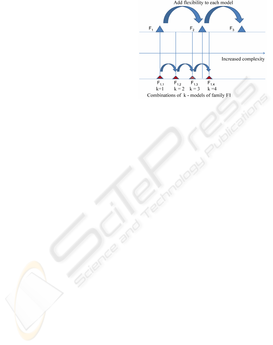
Figure 1 shows a diagram illustrating our main
ideas. Traditional approaches to model selection vary
complexity by jumping between model families F
i
;
every single model in the new family is able to create
more flexible decision boundaries compared to any
single model in the first family. Alternatively, com-
plexity can vary by combining multiple models into
a composite model (while fixing the complexity of
each single model in the first family); every model in
the new family F
ik
is the result of combining k mod-
els from the first family F
i
. New models are also
more complex but due to the composite approach.
The question is how do these two approaches com-
pare? How much complexity is precisely increased
with each approach? When combining k models, how
far can k increase until complexity grows above the
traditional approach of invoking single complex mod-
els? By answering these questions we open the possi-
bility of including both approaches in the same model
selection strategy, while expanding our understanding
of learning-algorithm designs.
This paper is organized as follows. Section 2
provides preliminary information in classification and
Structural Risk Minimization. Section 3 is a concep-
tual study that compares a composite model made of
multiple local models vs one single model. Finally,
section 4 gives a summary and discusses future work.
2 PRELIMINARIES
2.1 Basic Notation in Classification
Let (A
1
, A
2
, ··· , A
n
) be an n-component vector-valued
random variable, where each A
i
represents an attribute
or feature; the space of all possible attribute vec-
tors is called the input space X . Let {y
1
, y
2
, ··· , y
k
}
be the possible classes, categories, or states of na-
ture; the space of all possible classes is called the
output space Y . A classifier receives as input a set
of training examples T = {(x, y)}, |T | = N, where
x = (a
1
, a
2
, ··· , a
n
) is a vector or point in the in-
put space and y is a point in the output space. We
Figure 1: Two types of model selection. Top: Complexity is
increased by looking at families of models F
i
with increased
flexibility in the decision boundaries. Bottom: Complexity
is increased by combining k models while fixing the com-
plexity of each model. F
ik
stands for the combination of k
models of family F
i
. If we could compare both approaches
–as in this example– we could say that model family F
13
is
less complex than family F
2
, which in turn is less complex
than family F
14
.
assume T consists of independently and identically
distributed (i.i.d.) examples obtained according to a
fixed but unknown joint probability distribution in the
input-output space X ×Y . The outcome of the classi-
fier is a function or model f mapping the input space
to the output space, f : X → Y . We consider the case
where a classifier defines a discriminant function for
each class g
j
(x), j = 1, 2, ··· , k and chooses the class
corresponding to the discriminant function with high-
est value (ties are broken arbitrarily):
f (x) = y
m
iff g
m
(x) ≥ g
j
(x) (1)
We work with kernel methods (particularly support
vector machines), where a solution to the classifica-
tion (or regression) problem uses a discriminant func-
tion of the form:
g(x) =
N
∑
i=1
α
i
K(x
i
, x) (2)
where {α
i
} is a set of real parameters, index i runs
along the number of training examples, and K is a
kernel function in a reproducing kernel Hilbert space
(Shawe-Taylor and Cristianini, 2004). We assume
polynomial kernels K(x
1
, x
2
) = (x
1
·x
2
)
p
, where p is
the degree of the polynomial.
ICAART 2010 - 2nd International Conference on Agents and Artificial Intelligence
114

3 A CONCEPTUAL STUDY
We now study the problem of model selection based
on the criterion proposed by Vapnik (Vapnik, 1999;
Hastie et al., 2001) under the name of Structural
Risk Minimization (SRM). Here the objective is
to minimize the expected value of a loss function
L(y, f (x)) that states how much penalty is assigned
when our class estimation f (x) differs from class y.
A typical loss function is the zero-one loss function
L(y, f (x)) = I(y 6= f (x)), where I(·) is an indicator
function. We define the risk in adopting a family of
models parameterized by θ as the expected loss:
R(θ) = E[L(y, f (x|θ))] (3)
which cannot be estimated precisely because y(x ) is
unknown. One can compute instead the empirical
risk:
ˆ
R(θ) =
1
N
N
∑
i=1
L(y
i
, f (x
i
|θ)) (4)
where N is the size of the training set. Using a mea-
sure of model-family complexity h, known as the VC-
dimension (Vapnik, 1999), the idea is now to provide
an upper bound on the true risk using the empirical
risk and a function that penalizes for complex models
using the VC dimension:
SRM:
R(θ) ≤
ˆ
R(θ) +
s
h(ln
2N
h
+ 1) −ln(
η
4
)
N
(5)
where the inequality holds with probability at least
1−η over the choice of the training set. The goal is to
find the family of models that minimizes equation 5.
The ideas just described are typical on model se-
lection techniques. Since our training set T comprises
a limited number of examples and we do not know
the form of the true target distribution, the problem
we face is referred to as the bias-variance dilemma
in statistical inference (Geman et al., 1992; Hastie
et al., 2001). Specifically, simple classifiers exhibit
limited flexibility on their decision boundaries; their
small repertoire of functions produces high bias (since
the best approximating function may lie far from the
target function) but low variance (since there is lit-
tle dependence on local irregularities in the data). In
such cases, it is common to see high values for the
empirical risk but low values for the penalty term. On
the other hand, complex models encompass a large
class of approximating functions; they exhibit flexi-
ble decision boundaries (low bias) but are sensitive to
small variations in the data (high variance). Here, in
contrast, we commonly find low values for the em-
pirical risk but high values for the penalty term. The
goal in SRM is to minimize the right hand side of in-
equality 5 by finding a balance between empirical er-
ror and model complexity, where the VC dimension h
becomes a controllable variable.
3.1 Multiple Models vs One Model
We now provide an analysis of the conditions under
which combining multiple local models is expected
to be beneficial. In essence we wish to compare a
composite model M
c
to a basic global model M
b
. M
c
is the combination of multiple models. We assume
M
b
has VC-dimension h
b
and M
c
has VC-dimension
h
c
, which comes from the combination of k models,
each of VC-dimension at most h, where we assume
h < h
b
.
The question we address is the following: how
many models of VC-dimension at most h can M
c
comprise to still improve on generalization accuracy
over M
b
, assuming both models have the same empir-
ical error? The question refers to the maximum value
of k that still gives an advantage of M
c
over M
b
. To
proceed we look at the VC-dimension of h
c
, which in
essence is the VC-dimension of k-fold unions or inter-
sections. It is an open problem to determine the VC-
dimension of a family of k-fold unions (Reyzin, 2006;
Blumer et al., 1989; Eisenstat and Angluin, 2007); re-
cent work, however, shows that such a family of mod-
els has a lower bound of
8
5
kh, and an upper bound of
2kh log
2
3k (it has been shown that O(nk log
2
k) is a
tight bound (Eisenstat and Angluin, 2007)). We be-
gin our study with the lower optimistic bound, and
assume the VC-dimension of h
c
to be
8
5
kh. To solve
the question above we equate the right hand side in
equation 5 for both M
c
and M
b
:
v
u
u
u
t
8
5
kh
ln
2N
8
5
kh
+ 1
−ln(
η
4
)
N
=
v
u
u
t
h
b
ln
2N
h
b
+ 1
−ln(
η
4
)
N
(6)
where our goal is now simply to solve for k. After
some algebraic manipulation we get the following:
c
1
k −k ln k = c
2
(7)
where c
1
and c
2
are constants:
c
1
= ln2N + 1 −ln(
8
5
h) (8)
A CONCEPTUAL STUDY OF MODEL SELECTION IN CLASSIFICATION - Multiple Local Models vs One Global
Model
115
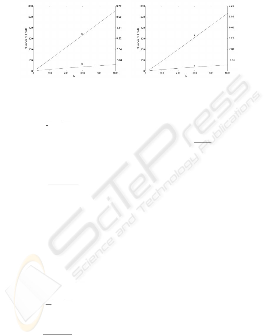
Figure 2: Left: A comparison of a compound model using k (k
0
) support vector machines with polynomial kernels of degree
one vs a simple support vector machine with a polynomial kernel of degree two; Right: same comparison except the simple
support vector machine has a polynomial kernel of degree four. The degree of the polynomial kernel makes little difference
in the results.
c
2
=
h
b
8
5
h
ln
2N
h
b
+ 1
(9)
Equation 7 can be formulated as a transcendental al-
gebraic equation. We can transform the equation as
follows:
−c
2
k
−1
e
−c
2
k
−1
= −c
2
e
−c
1
(10)
To solve for k we can use Lambert’s W function:
k =
−c
2
W (−c
2
e
−c
1
)
(11)
where W can be solved using a numeric approxima-
tion.
A similar analysis can be done using the upper
bound of h
c
= 2k
0
hlog
2
3k
0
, where we use k
0
to dif-
ferentiate from the k used with the lower bound. Af-
ter some algebraic manipulation we get the following
equation:
c
3
ν −ν ln ν = c
4
(12)
where ν = k
0
ln3k
0
, and c
3
and c
4
are constants (only
slightly different than before):
c
3
= ln2N + 1 −ln(
2h
ln2
) (13)
c
4
=
h
b
2h
ln2
ln
2N
h
b
+ 1
(14)
Since equations 7 and 12 have the same form, ν has
the same solution as k (equation 11):
ν =
−c
4
W (−c
4
e
−c
3
)
= c
5
(15)
We can then do the substitution back to k
0
to obtain
the following:
k
0
ln3k
0
= c
5
(16)
c
5
(k
0
)
−1
e
c
5
(k
0
)
−1
= 3c
5
(17)
It is now possible to solve for k
0
:
k
0
=
c
5
W (3c
5
)
(18)
To summarize, we have shown how to express the
number of k-fold (and k
0
-fold) unions of models, each
with VC-dimension h, such that the resulting com-
pound model exhibits the same guaranteed risk as
a single model with VC-dimension h
b
(we assume
of course that h < h
b
). To clarify, we handle two
bounds, k and k
0
, because of our uncertainty in the
VC-dimension of model unions. In principle we know
there is a k
00
, that stands as the exact bound, below
which M
c
retains an advantage over M
b
.
We can now study the effect on k (and k
0
) as we
vary parameters such as the size of the training set,
or the VC-dimension of the models in the compos-
ite model M
c
(as compared to the global model M
b
).
Figures 2 and 3 show plots on how the number of
model unions varies with different values of N. In
each case we take the compound model as the union
of k (and k
0
) support vector machines, where the sim-
ple global model is a single support vector machine.
We assume the use of polynomial kernels where the
VC-dimension of each model is defined as (Burges,
1998):
h =
n + p −1
p
+ 1 (19)
where n is the dimensionality of the input space and
p is the degree of the polynomial. In Figure 2 we as-
sume a compound model with polynomial kernels of
degree p = 1. The global model varies from a poly-
nomial degree p = 2 (Figure 2-left) to a polynomial
degree p = 4 (Figure 2-right). In all cases we as-
sume n = 5. It is clearly observed that the value of
ICAART 2010 - 2nd International Conference on Agents and Artificial Intelligence
116
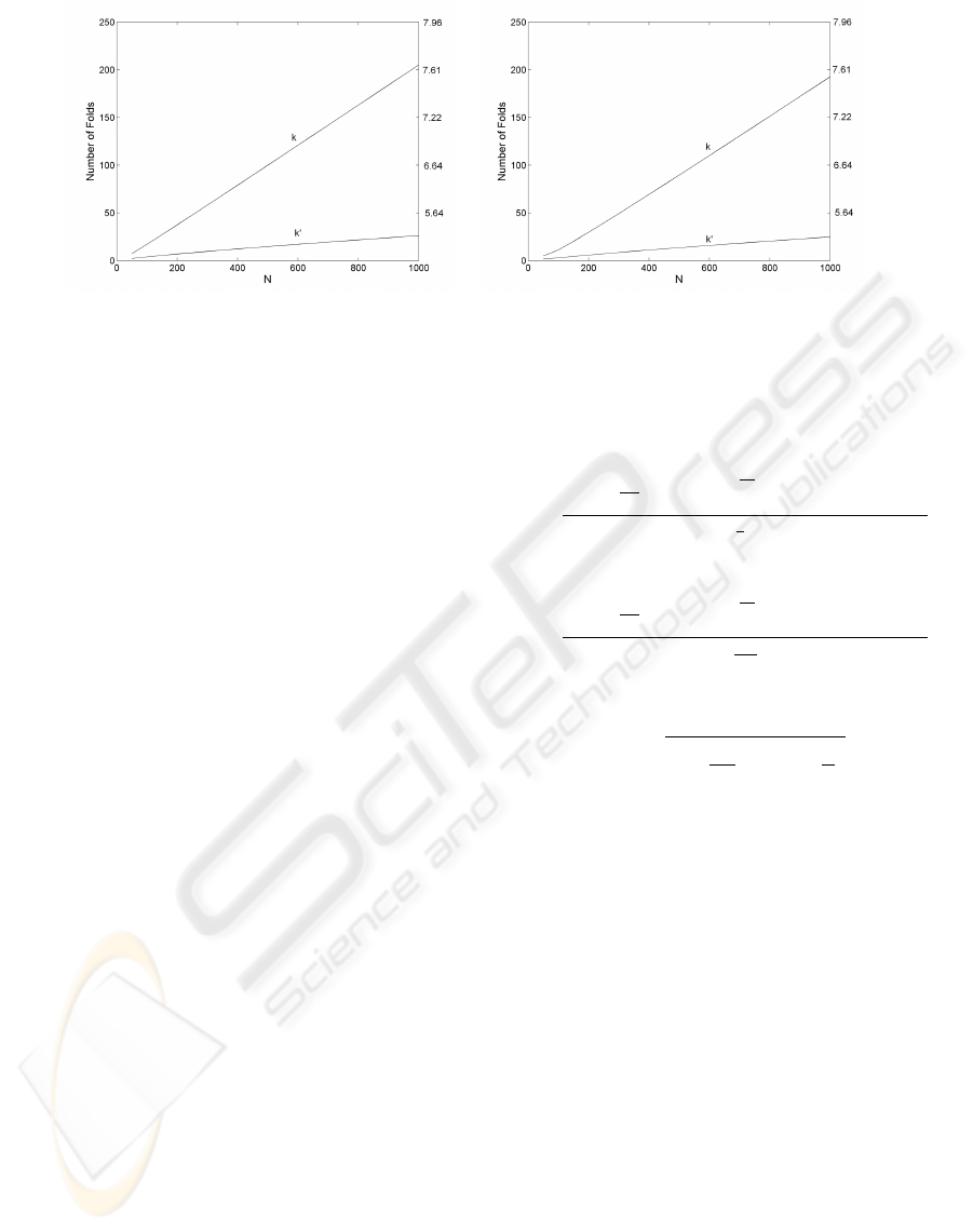
Figure 3: Left: A comparison of a compound model using k (k
0
) support vector machines with polynomial kernels of degree
two vs a simple support vector machine with a polynomial kernel of degree three; Right: same comparison except the simple
support vector machine has a polynomial kernel of degree five. The degree of the polynomial kernel makes little difference in
the results.
k (k
0
) increases linearly with N. As expected, k
0
cor-
responds to a less inclined line as the upper bound on
the VC-dimension lowers the number of models we
can place at the composite model while still gener-
ating less variance as the single model. In addition,
a higher difference in VC-dimension (Figure 2-right)
shows almost no difference in the shape of k (k
0
) for
different values of N. The right y-axis on each graph
is the log
2
of the values on the left y-axis; it is sim-
ply an indicator of how many local models we could
arrange in a hierarchical structure (assuming a binary
tree) while still generating less variance as the global
model. We observe that for large values of N (e.g.,
N > 500), large hierarchies can be employed with lit-
tle effect over the variance component.
Figure 3 assumes a compound model with poly-
nomial kernels of degree p = 2. The single model
varies from a polynomial degree p = 3 (Figure 3-
left) to a polynomial degree p = 5 (Figure 3-right).
The same effect is observed as before except under
a different scale. In all graphs we observe a large
advantage gained by the combination of many low-
complex models as compared to a single model ex-
hibiting higher complexity. The difference grows lin-
early on N and is considerable for N > 500.
Until now we have assumed the empirical error to
be the same for the compound model M
c
and for the
global model M
b
. We now analyze the case where
empirical errors differ. Let
ˆ
R
c
(θ) be the empirical
error for M
c
and
ˆ
R
b
(θ) the corresponding error for
M
b
; we define the difference in empirical error as
∆
ˆ
R(θ) =
ˆ
R
c
(θ) −
ˆ
R
b
(θ), and ask the same question as
before, how many models of VC-dimension at most
h can M
c
comprise to still improve on generalization
accuracy over M
b
? This time, however, we account
for differences in empirical error. Our previous anal-
ysis remains almost the same. We need only make a
modification on two constants:
c
2
=
h
b
ln
2N
h
b
+ 1
−2
√
N∆
ˆ
R(θ)Ψ + N∆
ˆ
R(θ)
2
8
5
h
(20)
c
4
=
h
b
ln
2N
h
b
+ 1
−2
√
N∆
ˆ
R(θ)Ψ + N∆
ˆ
R(θ)
2
2h
ln2
(21)
where
Ψ =
r
h
b
ln
2N
h
b
+ 1 −ln(
η
4
) (22)
Figure 4 shows plots on how the number of model
unions varies with different values of ∆
ˆ
R(θ) when
N = 500 and the confidence level is set to η = 0.05.
Here we assume a compound model with polynomial
kernels of degree p = 1 and a global model with a
polynomial kernel of degree p = 2. Figure 4-left
shows the case when n = 5 and Figure 4-right shows
the case when n = 15. Surprisingly, error differences
have little effect on the value of the number of folds.
We also observe that an increase in the dimensional-
ity of the space imposes a tighter bound on the num-
ber of combined models (it adds weight to the VC-
dimension of every model).
Overall we conclude that adding complexity to a
single model is equivalent to making long steps in
increasing model variability (as determined by the
penalty term in equation 5). Smaller steps can be
achieved through the union of simple models. Even
when it is known that the bounds derived from the
principle of SRM are not tight, the number of sim-
ple models that can be combined before reaching the
equivalent effect of a single but more complex model
is significantly large.
A CONCEPTUAL STUDY OF MODEL SELECTION IN CLASSIFICATION - Multiple Local Models vs One Global
Model
117
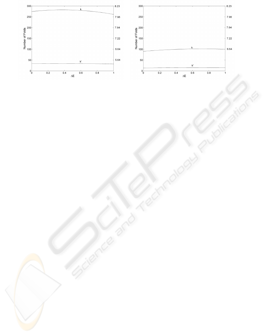
Figure 4: A comparison of a compound model using k (k
0
) support vector machines with polynomial kernels of degree one
vs a simple support vector machine with a polynomial kernel of degree two. The x-axis refers to the difference in empirical
error, ∆E = ∆
ˆ
R(θ) =
ˆ
R
c
(θ) −
ˆ
R
b
(θ), between the compound model and the global model. Left: number of dimensions n = 5.
Right: number of dimensions n = 15.
4 SUMMARY AND FUTURE
WORK
Our study compares the bias-variance tradeoff of a
model that combines several simple classifiers with
a single more complex classifier. Using standard
bounds for the actual risk (using the VC-dimension),
a single increase in the polynomial degree of the ker-
nel function for a support vector machine increases
the variance component significantly. As a result,
multiple simple classifiers can be combined before
the compound model exceeds the variance of a sin-
gle more complex classifier.
Our study advocates a piece-wise model fitting ap-
proach to classification, justified by the difference in
the rate of complexity obtained by augmenting the
number of boundaries per class (composite model)
to the increase in complexity obtained by augment-
ing the capacity of a single global learning algorithm
(classical approach). The former enables us to in-
crease the model complexity in finer steps.
As future work we plan on extending our study to
hierarchical learning, where a data structure defined a
priori over the application domain explicitly indicates
how classes divide into more specific sub-classes. A
hierarchical classification model can be seen as the
composition of many models, one for each node in
the hierarchy. Our study can be used to compare hier-
archical models with single global models by taking
into account the increase in variance gained by reduc-
ing the size of the training set as each lower hierarchi-
cal node covers a smaller number of examples.
ACKNOWLEDGEMENTS
This work was supported by National Science Foun-
dation under grants IIS-0812372 and IIS-0448542,
and by the Army Research Office under grant
56268NSII. F. Ocegueda-Hernandez was supported
by CONACyT (Mexico), Ph.D. fellowship 171936.
REFERENCES
Blumer, A., Ehrenfeucht, A., Haussler, D., and Warmuth,
M. (1989). Learnability and the vapnik-chervonenkis
dimension. Journal of the ACM, 36(4):929–965.
Burges, C. J. C. (1998). A tutorial on support vector
machines for pattern recognition. Data Mining and
Knowledge Discovery, 2(2):121–167.
Eisenstat, D. and Angluin, D. (2007). The vc dimen-
sion of k-fold union. Information Processing Letters,
101(5):181–184.
Geman, S., Bienenstock, E., and Doursat, R. (1992). Neu-
ral networks and the bias/variance dilemma. Neural
Computation, 4(1):1–58.
Hastie, T., Tibshirani, R., and Friedman, J. (2001). The Ele-
ments of Statistical Learning: Data Mining, Inference,
and Prediction. Springer.
Kearns, M., Mansour, Y., Ng, A., and Ron, D. (1997). An
experimental and theoretical comparison of model se-
lection methods. Machine Learning, 27(1):7–50.
Reyzin, L. (2006). Lower bounds on the vc dimen-
sion of unions of concept classes. Technical Re-
port, Yale University, Department of Computer Sci-
ence, YALEU/DCS/TR-1349.
Shawe-Taylor, J. and Cristianini, N. (2004). Kernel Meth-
ods for Pattern Analysis. Cambridge University Press.
Vapnik, V. (1999). The Nature of Statistical Learning The-
ory. Springer, 2nd edition.
ICAART 2010 - 2nd International Conference on Agents and Artificial Intelligence
118
