HANDLING DYNAMIC MULTIOBJECTIVE PROBLEMS WITH

PARTICLE SWARM OPTIMIZATION

Alan D

ıaz Manr

ıquez, Gregorio Toscano Pulido and Jos

e Gabriel Ram

ırez Torres

Laboratorio de Tecnolog

ıas de Informaci

on, CINVESTAV-Tamaulipas

Km. 6 carretera Cd. Victoria-Monterrey. Cd. Victoria, Tamaulipas, 87267, Mexico

Keywords:

Dynamic multi-objective optimization, Particle swarm optimization, Multi-objective optimization.

Abstract:

In this paper the hyperplane distribution and Pareto dominance were incorporated into a particle swarm op-

timization algorithm in order to allow it to handle dynamic multiobjective problems. When a change in a

dynamic multiobjectve function is detected, the proposed algorithm reinitializes (in different ways) the PSO’s

velocity parameter and the archive where the non-dominated solutions are beeing stored such that the algorithm

can follow the dynamic Pareto front. The proposed approach is validated using two dynamic multiobjective

test functions and an standard metric taken from the specialized literature. Results indicate that the proposed

approach is highly competitive which can be considered as a viable alternative in order to solve dynamic

multiobjective optimization problems.

1 INTRODUCTION

Since life is dynamic, it is only natural to expect that

the problems from daily life are dynamics. Robot path

planning, or the selection of routes in a communica-

tions network are some problems whose function ﬂuc-

tuates over time or incorporates some kind of noise.

These problems are called “non-stationary” or “dy-

namic”.

A dynamic optimization problem (DOP) may in-

volve two or more functions to be optimized simulta-

neously (also known as dynamic multiobjective op-

timization problems, or DMOP for short), as well

as constraints and parameters which can be changed

over time. Dealing with a DMOP increases the com-

plexity of a dynamic problem, since it is imperative

to detect the change in order to re-evaluate the previ-

ously stored solutions. Also, it can increase the num-

ber of objective functions, and therefore the optimiza-

tion process may change dramatically.

Although the study of this type of problems is not

new, most of the proposed approaches transform the

original dynamic problem into many static optimiza-

tion problems. The scientiﬁc community of evolu-

tionary computation has focused their efforts on de-

signing approaches to manage a set of valid solu-

tions (population) to solve these problems without

performing any transformation. The resulting ap-

proaches can take advantage of previous knowledge

to direct the search.

Kennedy and Eberhart proposed an approach

called “Particle Swarm Optimization” (PSO) which

was inspired on the choreography of a bird ﬂock. Like

other evolutionary algorithms, PSO uses a set of pos-

sible solutions which will be “evolved” until an opti-

mal solution or a termination criteria is reached. In

this case, each solution (x) is represented by a parti-

cle, and a set of particles are represented by a swarm.

The responsibility of evolving (moving) the swarm to

the optimal region corresponds to the velocity equa-

tion. This equation is usually composed by three

elements: a velocity inertia, a cognitive component

(pbest) and a social component (gbest). The entire

approach can be seen as a distributed behavioral al-

gorithm that performs (in its more general version) a

multidimensional search. In the simulation, the be-

havior of each particle is affected by either the best

local particle (i.e., within a certain neighborhood) or

the best global particle (Kennedy and Eberhart, 2001).

An interesting aspect of PSO is that it allows in-

dividuals to beneﬁt from their past experiences (note

that in other approaches such as the genetic algorithm,

normally the current population is the only “memory”

used by the individuals).

The remain of this paper is organized as follows:

Basic concepts are given in Section 2. In Section 3,

we present the dynamic multiobjective state-of-the-

art. Section 4 describes the proposed algorithm and

337

Díaz Manríquez A., Toscano Pulido G. and Gabriel Ramírez-Torres J. (2010).

HANDLING DYNAMIC MULTIOBJECTIVE PROBLEMS WITH PARTICLE SWARM OPTIMIZATION.

In Proceedings of the 2nd International Conference on Agents and Artiﬁcial Intelligence - Artiﬁcial Intelligence, pages 337-342

DOI: 10.5220/0002734403370342

 SciTePress

the components that it is conformed by. Section 5

presents the experiments and the comparison of re-

sults. Finally, Section 6 provides the concluding re-

marks and future work.

2 BASIC CONCEPTS

Deﬁnition 1 (Dynamic Multiobjective Optimiza-

tion Problem (DMOP)). Find ~x which minimizes:

f (~x,t) = [ f

(~x,t), f

(~x,t),..., f

(~x,t)]

, subject to m

inequality constraints: g

(~x,t) ≤ 0 i =

1,2, ...,m, and p equality constraints: h

(~x,t) =

0 j = 1, 2,..., p, where ~x is the vector of

decision variables;

f is the set of objective functions

to be minimized in time t. The functions g and h, rep-

resent the set of constraints, that deﬁne the feasible

region F in time t. 

Deﬁnition 2 (Pareto Optimality). A point ~x

∗

∈ F

is Pareto optimal in time t, if for every ~x ∈ F and I =

{1,2, .. ., k} either, ∀

i∈I

( f

(~x,t) = f

(~x

∗

,t)) or, there is

at least one i ∈ I such that f

(~x,t) > f

(~x

∗

,t) 

Deﬁnition 3 (Pareto Dominance). A vector ~x =

,. .. ,x

]

is said to dominate ~y = (y

,. .. ,y

) (de-

noted by~x ~y) if and only if x is partially less than y,

i.e., ∀i ∈ {1, .. ., k}, x

≤ y

∧ ∃i ∈ {1,. . ., k} : x

< y



Deﬁnition 4 (Pareto-Optimal Set). For a given

time t and a given MOP

f (x,t), the Pareto optimal set

∗

) is deﬁned as:

:= {x ∈ F | @ x

∈ F

f (x

,t) 

f (x,t)}. (1)



Deﬁnition 5 (Pareto Front). For a given MOP

f (x,t), and Pareto optimal set P

, in time t, the Pareto

front (P F

) is deﬁned as:

P F

∗

:= {~u =

f = ( f

(x,t), .. ., f

(x,t)) | x ∈ P

∗

(2)



In the general case, it is impossible to ﬁnd an an-

alytical expression of the line or surface that contains

these points. The normal procedure to generate the

Pareto front is to compute the feasible points F and

their corresponding f (F ). When there is a sufﬁcient

number of these, it is then possible to determine the

non-dominated points and to produce the Pareto front.

Furthermore, DMOP can be clustered into four

types (Farina et al., 2004):

• Type I. Change on the Pareto-optimal set (P

whereas the Pareto-optimal front (optimal objec-

tive values) (P F

) does not change.

• Type II. Both P

and P F

change.

• Type III. P

does not change, whereas P F

changes.

• Type IV. Both P

and P F

do not change, al-

though the problem can dynamically change (e.g.,

the constraints can vary).

Since Types II and III are the most challenging

type of DMOP, we focused in solving these kind of

problems.

3 RELATED WORK

Evolutionary algorithms have been successfully ap-

plied to solve DMOPs. Their succeed might be di-

rected by their population-based nature, since this

allows to use the most of the previous discovered

knowledge in order to follow the change in the en-

vironment.

Bingul (Bingul, 2007) solved a dynamic multiob-

jective optimization problem (DMOP) using an ag-

gregating function approach with a Genetic Algo-

rithm (GA). Zeng et al. (Zeng et al., 2006) intro-

duced a dynamic orthogonal multiobjective evolu-

tionary called DMOEA. Their approach selects ran-

domly between an orthogonal crossover operator and

a linear crossover operator. The ﬁrst operator was

proposed with the aim to enhance the ﬁtness of the

population while the process is stabilized between

two changes. Hatzakis and Wallace (Hatzakis and

Wallace, 2006) proposed a forward-looking approach

which combines a forecasting technique with an evo-

lutionary algorithm. Deb et al. (Deb et al., 2000)

proposed two modiﬁcations to the NSGA-II in order

to be able to handle DMOPs. In the ﬁrst modiﬁca-

tion, the population is reinitialized whilst in the sec-

ond the population is hyper-mutated depending on the

type of change in the environment (Deb et al., 2006).

Talukder and Kirley (Talukder and Kirley, 2008) used

a new variation operator to follow the Pareto front in

DMOPs. Zhou et al. (Zhou et al., 2006) proposed

two strategies to perform a population re-initialization

when a change in the environment is detected. Wang

and Dang transform the objectives of the original

DMOP in a set of static bi-objective (Yuping Wang,

2008). Ray et al. (Ray et al., 2009) introduced a

memetic algorithm which employs an orthogonal ε-

constrained formulation to deal with multiple objec-

tives and a sequential quadratic programming (SQP)

ICAART 2010 - 2nd International Conference on Agents and Artificial Intelligence

338

solver is embedded as its local search mechanism in

order to improve the convergence rate.

4 PROPOSED APPROACH

PSO has been successfully used for both continuous

nonlinear and discrete binary single objective opti-

mization (Kennedy and Eberhart, 2001). The pseu-

docode of the PSO pseudocode is shown in Algorithm

Algorithm 1. PSO Algorithm.

gbest ← ~x

for i = 0 to nparticles do

pbest

← ~x

← initialize randomly()

f itness

← f (~x

)

if f itness

< f (

gbest) then

gbest ← ~x

end if

end for

repeat

for i = 0 to nparticles do

for d = 0 to ndimensions do

← W ∗ v

+ C

∗ U (0,1) ∗ (pbest

− x

) + C

∗ U (0,1) ∗

(gbest − x

)

← x

+ v

end for

f itness

← f (~x

)

if f itness

< f (

pbest

) then

pbest

← ~x

end if

if f itness

< f (

gbest

) then

gbest

← ~x

end if

end for

until Termination criterion

4.1 Handling Multiple Dynamic

Objectives with PSO

PSO seems particularly suitable for dynamic multiob-

jective optimization mainly because of the high speed

of convergence that the algorithm presents for single-

objective optimization. Based on such behavior, one

would expect that a multiobjective PSO (MOPSO) to

be very efﬁcient computationally speaking. However,

in order to be able to handle dynamic multiobjective

problems there is necessary to perform three main

modiﬁcations to the original algorithm.

• To modify the algorithm to handle multiple ob-

jectives and produce a set of non-dominated solu-

tions in a single run.

• To modify the algorithm to obtain a good distribu-

tion of solutions.

• To modify the algorithm in order to handle its be-

havior when a change is detected.

A natural modiﬁcation to a PSO algorithm aimed

handle multiple objectives is replace the comparison

operator in order to determine whether a solution a

is better a solution b. The analogy of particle swarm

optimization with evolutionary algorithms makes ev-

ident the notion that using a Pareto ranking scheme is

a straightforward way to extend the approach to han-

dle multiobjective optimization problems. However,

if we merge a Pareto ranking scheme with the PSO al-

gorithm a set of non-dominated solutions will be pro-

duced (by deﬁnition, all non-dominated solutions are

equally good). Having several non-dominated solu-

tions implies the inclusion into the algorithm of both:

an additional criteria to decide whether a new non-

dominated solution is pbest or gbest and a strategy to

select the guide particles (pbest and gbest).

In order to select an strategy to choose the gbest

solution, we performed three experiments:

1. To choose randomly among all the particles in the

archive.

2. To choose the non-dominated particle closer to

pbest.

3. To choose the non-dominated particle more dis-

tant to the pbest.

Experimental results indicate us that the best strat-

egy to select the gbest was: 1) random selection.

Several approaches have suggest that the use of

elitism by means of an external archive in order to

store the non-dominated solutions can enable most al-

gorithms to ﬁnd the Pareto front. However, the size

of the archive can grow very fast, and therefore, it is

imperative to maintain a small set of non-dominated

solutions. We selected the hyper-plane distribution

algorithm in order to maintain diversity and to re-

duce the size of non-dominated solutions stored in the

archive(Blinded, 2005).

4.2 Hyper-plane Distribution

The core idea of this proposal is to perform a good

distribution of the hyper-plane space deﬁned by the

minima (assuming minimization) from the objectives,

and use such distribution to select a representative

subset from the whole set of non-dominated solutions.

The algorithm works as follows: First it accepts a set

of non-dominated vectors and a number n of solutions

of the desirable subset as its input. Then, the algo-

rithm selects those vectors which have the minimum

and maximum value of each objective, and it groups

them into two sets, the minima set (called MIN), and

HANDLING DYNAMIC MULTIOBJECTIVE PROBLEMS WITH PARTICLE SWARM OPTIMIZATION

339

the maxima set (called MAX). Using MIN, the algo-

rithm creates a hyper-plane, and distributes its space

into n − 1 ﬁxed-size sub hyper-planes. After that, it

computes lines on each subdivision; such lines are

perpendicular to the hyper-plane. Finally, the algo-

rithm returns the closest vectors to each line.

4.3 Adaption to the Change

Since the natural behavior of a DMOP is to be chang-

ing, it is essential that the algorithm performs a good

reaction when a change is detected. Therefore, in or-

der to properly follow the Pareto Front, we need to

reinitialize the PSO algorithm. However, such reini-

tialization can be made using four strategies:

• DPSO-1. The current solution (after the change)

will be taken as pbest. The particles are reeval-

uated and the resulting non-dominated solutions

are stored in the archive.

• DPSO-2. This is similar to DPSO-1. However, in

this strategy, the archive will be updated using the

hyper-plane distribution.

• DPSO-3. Similar to DPSO-1, but the velocity of

each particle will be reinitialized to zero.

• DPSO-4. This strategy is similar to DPSO-2, but

this strategy reinitializes the velocity of each par-

ticle (to zero).

5 EXPERIMENTS AND

COMPARISON OF RESULTS

Two test functions were taken from the specialized

literature to compare our approaches. In order to al-

low a quantitative assessment of the performance of

a multiobjective optimization algorithm, the Inverted

Generational Distance (IGD) metric was adopted.

Inverted Generational Distance (IGD): The

concept of generational distance was introduced by

Van Veldhuizen & Lamont (Veldhuizen and Lamont,

1998; Veldhuizen and Lamont, 2000) as a way of es-

timating how far are the elements in the Pareto front

produced by our algorithm from those which belongs

to the true Pareto front of the problem. This measure

is deﬁned as:

GD =

∑

i=1

(3)

where n is the number of non-dominated vectors

found by the algorithm being analyzed and d

is the

Euclidean distance (measured in objective space) be-

tween each of these and the nearest member of the

true Pareto front. It should be clear that a value of

GD = 0 indicates that all the elements generated are

in the true Pareto front of the problem.

In order to know how competitive is our approach,

we decided to compare our results with respect to

those obtained by the NSGA II-A and the NSGA II-B

(Deb et al., 2006), these algorithms use the parame-

ter ζ that is the percentage of population which will

be reinitialized in the NSGA II-A and hyper-mutated

in the NSGA II-B, this variation operators would be

applied when a change is detected.

In all the following examples, we report the results

obtained from 100 independent runs of each com-

pared algorithm.

In order to have a fair comparison, we hand-tune

each change to be activated every 500 evaluations of

the objective function. For such sake, we setup the

population of NSGA II-A and NSGA II-B to 52 in-

dividuals and τ

= 10 , n

= 10, and ζ = 20%. The

DPSO-1, DPSO-2, DPSO-3 and DPSO-4 were exe-

cuted using 20 particles, the size of the archive was

n = 100, and the parameters W = 0.4 and C

= C

1.49.

The tests functions used for the algorithms are

shown in the Table 1.

Table 1: Tests functions.

FDA1

) = x

,g(X

) = 1 +

∑

∈X

− G(t))

h( f

,g) = 1 −

,G(t) = sin(0.5πt)

= g ∗h( f

,g)

t =

τ is the generation counter and τ

is the number

of generations that t is ﬁxed.

= (x

)

∈ [0, 1], X

= (x

,..., x

)

,..., x

∈ [−1, 1]

FDA2

mod

) = x

,g(X

) = 1 +

∑

∈X

h(X

III

, f

,g) = 1 −

e(t,X

III

)

H(t) = 0.2 + 4.8t

,t =

= g ∗h( f

,g)

τ is the generation counter τ

is the number

of generations that t is ﬁxed.

= (x

)

∈ [0, 1], X

∈ [−1, 1]

III

=∈ [−1, 1]

,1 +r

+ r

= n

The algorithms were executed until 10 changes

have occurred in each test function. However, since

there is a large amount of data, it would be very con-

fused to display it in a numerical mode. Therefore, in

order to presente the results in a more compact way,

we decided to use box-plot graphics of the application

of the IGD metric to the Pareto known before each

change.

ICAART 2010 - 2nd International Conference on Agents and Artificial Intelligence

340

●●●

●

●●●

●●

●●●

●

●●●

●●

●

●●●

●

●●●

●●

●●●

●●

●●●

●

●●

●

●●●

●

●●●

●

●●

●

●●●

●

●●

●

●●

●

1 2 3 4 5 6 1 2 3 4 5 6 1 2 3 4 5 6 1 2 3 4 5 6 1 2 3 4 5 6

0.0 0.5 1.0 1.5 2.0

RGD

Change 0 Change 1 Change 2 Change 3 Change 4

●

●●●

●

●●

●

●●

●

●●●

●

●●

●

●●

●

●●

●●●

●

●●●

●●

●

●●

●

●●

●

●●●

●

●●

●

1 2 3 4 5 6 1 2 3 4 5 6 1 2 3 4 5 6 1 2 3 4 5 6 1 2 3 4 5 6

0.0 0.5 1.0 1.5 2.0

RGD

Change 5 Change 6 Change 7 Change 8 Change 9

(a) Inverted generational distance results for FDA1

●

●●

●

●●

●

●●

●

●●

●

1 2 3 4 5 6 1 2 3 4 5 6 1 2 3 4 5 6 1 2 3 4 5 6 1 2 3 4 5 6

0.0 0.5 1.0 1.5 2.0

RGD

Change 0 Change 1 Change 2 Change 3 Change 4

●

●●

●

●●●

●●

●

●●●

●●

●●●

●●

●

●●●

●

●●

●

●●●

●●

●

●●●

●●

●●●

●●

●

●●●

●

●●

●

●●●

●●

●

●●●

●●

●●●

●●

●

●●●

●

●●

●

●●●

●●

●

●●●

●●

●●●

●●

●

●●●

●

●●

●

●●●

●●

●

●●

●

1 2 3 4 5 6 1 2 3 4 5 6 1 2 3 4 5 6 1 2 3 4 5 6 1 2 3 4 5 6

0.0 0.5 1.0 1.5 2.0

RGD

Change 5 Change 6 Change 7 Change 8 Change 9

(b) Inverted generational distance results for FDA2

mod

Figure 1: Box-plot of the application of the inverted gener-

ational distance metric to the results produced 100 indepen-

dent runs by 1) DPSO-1, 2) DPSO-2, 3) DPSO-3, 4) DPSO-

4, 5) NSGA II-A and 6) NSGA II-B for both test functions:

(a) and (b) refers to the inverted generational distance for

FDA1 and FDA2, respectively.

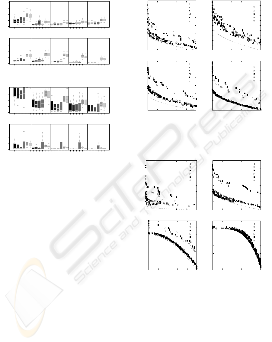
Results obtained when FDA1 was optimized show

that all versions of DPSO and the NSGA II-A and

NSGA II-B behaved similarly. Results from IGD sug-

gest, that all versions of DPSO had a better a conver-

gence than NSGA II-A and NSGA II-B (see Figure

1(a)). When comparing the DPSO versions, we can

say that the best performance were for those solutions

algorithm that preserve the velocity value before the

change (those who did not initialized the velocity to

0). Also, in Figure 5, we can see the Pareto fronts pro-

duced by the different algorithms. From this ﬁgure, it

is clear that DPSO outperforms the NSGA II-A and

NSGA II-B.

The results obtained for FDA2

mod

show that all

versions of DPSO and the NSGA II-A and NSGA II-

B also behaved similar. However, from the IGD met-

ric shown in Figure 1(b), we can easily observed that

the results from all versions of DPSO outperform to

those solutions obtained by NSGA II-A and NSGA

II-B. When comparing the DPSO versions, we can

say that the reinitialization of the velocity plays a key

role in the algorithm. Such that, in the initial changes

of the ﬁtness function, the algorithms which did not

0.5

1.5

2.5

0 0.2 0.4 0.6 0.8 1

DPSO-1

DPSO-2

DPSO-3

DPSO-4

NSGA2-A

NSGA2-B

FDA1

0.2

0.4

0.6

0.8

1.2

1.4

1.6

1.8

0 0.2 0.4 0.6 0.8 1

DPSO-1

DPSO-2

DPSO-3

DPSO-4

NSGA2-A

NSGA2-B

FDA1

0.5

1.5

2.5

0 0.2 0.4 0.6 0.8 1

DPSO-1

DPSO-2

DPSO-3

DPSO-4

NSGA2-A

NSGA2-B

FDA1

0.5

1.5

2.5

0 0.2 0.4 0.6 0.8 1

DPSO-1

DPSO-2

DPSO-3

DPSO-4

NSGA2-A

NSGA2-B

FDA1

Figure 2: Pareto fronts produced by all versions of DPSO,

NSGA II-A and NSGA II-B for FDA1 test function: change

1 is shown in the top left; change 3 is shown in the top right,

change 6 is shown in the bottom left, change 9 is shown in

the bottom right.

0 0.2 0.4 0.6 0.8 1

DPSO-1

DPSO-2

DPSO-3

DPSO-4

NSGA2-A

NSGA2-B

FDA2mod

0.5

1.5

2.5

0 0.2 0.4 0.6 0.8 1

DPSO-1

DPSO-2

DPSO-3

DPSO-4

NSGA2-A

NSGA2-B

FDA2mod

0.2

0.4

0.6

0.8

1.2

1.4

0 0.2 0.4 0.6 0.8 1

DPSO-1

DPSO-2

DPSO-3

DPSO-4

NSGA2-A

NSGA2-B

FDA2mod

0.2

0.4

0.6

0.8

1.2

0 0.2 0.4 0.6 0.8 1

DPSO-1

DPSO-2

DPSO-3

DPSO-4

NSGA2-A

NSGA2-B

FDA2mod

Figure 3: Pareto fronts produced by all versions of DPSO,

NSGA II-A and NSGA II-B for FDA2

mod

test function:

change 1 is shown in the top left; change 3 is shown in the

top right, change 6 is shown in the bottom left, change 9 is

shown in the bottom right.

reinitialize the velocity (to zero), obtained better re-

sults.

6 CONCLUSIONS

We have presented a proposal to extend particle

swarm optimization to handle dynamic multiobjective

HANDLING DYNAMIC MULTIOBJECTIVE PROBLEMS WITH PARTICLE SWARM OPTIMIZATION

341

problems. The proposed approach was validated us-

ing the standard methodology currently adopted for

the evolutionary multiobjective optimization commu-

nity. Results indicate that our approach is a viable al-

ternative since its performance is highly competitive

with respect to some of the best dynamic multiobjec-

tive evolutionary algorithms known-to-date.

One aspect that we would like to explore in the fu-

ture is to study how the DPSO behaves with a differ-

ent the particles’ interconnection topology. Further-

more, we would like to explore the use of different

values for W , C1, and C2.

ACKNOWLEDGEMENTS

Acknowledgements The ﬁrst author acknowledges

support from CONACyT through a scholarship to

pursue graduate studies at the Information Tech-

nology Laboratory at CINVESTAV-IPN. The sec-

ond author gratefully acknowledges support from

CONACyT through project 90548. Also, This re-

search was partially funded by project number 51623

from “Fondo Mixto Conacyt-Gobierno del Estado de

Tamaulipas”. Finally, we would like to thank to

Fondo Mixto de Fomento a la Investigaci

on cient

ıﬁca

y Tecnol

ogica CONACyT - Gobierno del Estado de

Tamaulipas for the support to publish this paper.

REFERENCES

Bingul, Z. (2007). Adaptive Genetic Algorithms Applied to

Dynamic Multi-ObjectiveProblems. Appl. Soft Com-

put., 7(3):791–799.

Blinded (2005). Blinded. PhD thesis, Blinded, Blinded.

Deb, K., Agrawal, S., Pratab, A., and Meyarivan, T. (2000).

A Fast Elitist Non-Dominated Sorting Genetic Al-

gorithm for Multi-Objective Optimization: NSGA-II.

KanGAL report 200001, Indian Institute of Technol-

ogy, Kanpur, India.

Deb, K., N., U. B. R., and Karthik, S. (2006). Dynamic

multi-objective optimization and decision-making us-

ing modiﬁed NSGA-II: A case study on hydro-thermal

power scheduling. In EMO, pages 803–817.

Farina, M., Deb, K., and Amato, P. (2004). Dynamic Mul-

tiobjective Optimization Problems: Test Cases, Ap-

proximations, and Applications. IEEE Transactions

on Evolutionary Computation, 8(5):425–442.

Hatzakis, I. and Wallace, D. (2006). Dynamic Multi-

Objective Optimization with Evolutionary Algo-

rithms: A Forward-Looking Approach. In et al.,

M. K., editor, 2006 Genetic and Evolutionary Compu-

tation Conference (GECCO’2006), volume 2, pages

1201–1208, Seattle, Washington, USA. ACM Press.

ISBN 1-59593-186-4.

Kennedy, J. and Eberhart, R. C. (2001). Swarm intelli-

gence. Morgan Kaufmann Publishers Inc., San Fran-

cisco, CA, USA.

Ray, T., Isaacs, A., and Smith, W. (2009). A memetic

algorithm for dynamic multiobjective optimization.

In Multi-Objective Memetic Algorithms, volume 171

of Studies in Computational Intelligence, pages 353–

367. Springer Berlin / Heidelberg.

Talukder, A. K. A. and Kirley, M. (2008). A pareto follow-

ing variation operator for evolutionary dynamic multi-

objective optimization. In Proceedings of the IEEE

Congress on Evolutionary Computation 2008 (CEC

2008), Hong Kong, China. IEEE Press, Piscataway,

NJ.

Veldhuizen, D. A. V. and Lamont, G. B. (1998). Multiob-

jective Evolutionary Algorithm Research: A History

and Analysis. Technical Report TR-98-03, Depart-

ment of Electrical and Computer Engineering, Gradu-

ate School of Engineering, Air Force Institute of Tech-

nology, Wright-Patterson AFB, Ohio.

Veldhuizen, D. A. V. and Lamont, G. B. (2000). On Mea-

suring Multiobjective Evolutionary Algorithm Perfor-

mance. In 2000 Congress on Evolutionary Computa-

tion, volume 1, pages 204–211, Piscataway, New Jer-

sey. IEEE Service Center.

Yuping Wang, C. D. (2008). An evolutionary algorithm for

dynamic multi-objective optimization. Applied Math-

ematics and ComputationIn Press.

Zeng, S., Chen, G., Zheng, L., Shi, H., de Garis, H., Ding,

L., and Kang, L. (2006). A Dynamic Multi-Objective

Evolutionary Algorithm Based on an Orthogonal De-

sign. In 2006 IEEE Congress on Evolutionary Com-

putation (CEC’2006), pages 2588–2595, Vancouver,

BC, Canada. IEEE.

Zhou, A., Jin, Y., Zhang, Q., Sendhoff, B., and Tsang, E.

(2006). Prediction-based population re-initialization

for evolutionary dynamic multi-objective optimiza-

tion. In Obayashi, S., Deb, K., Poloni, C., Hiroyasu,

T., and Murata, T., editors, The 4th Int. Conf. on Evo-

lutionary Multi-Criterion Optimization, volume 4403,

pages 832–846. Springer.

ICAART 2010 - 2nd International Conference on Agents and Artificial Intelligence

342