
ON AMBIGUITY DETECTION AND POSTPROCESSING SCHEMES
USING CLUSTER ENSEMBLES
Amparo Albalate, Aparna Suchindranath, Mehmet Muti Soenmez
Institute of Information Technology, University of Ulm, Germany
David Suendermann
SpeechCycle Labs, NY, U.S.A.
Keywords:
Cluster ensembles, Uncertainty, Ambiguity.
Abstract:
In this paper, we explore the cluster ensemble problem and propose a novel scheme to identify uncer-
tain/ambiguous regions in the data based on the different clusterings in the ensemble. In addition, we analyse
two approaches to deal with the detected uncertainty. The first, simplest method, is to ignore ambiguous pat-
terns prior to the ensemble consensus function, thus preserving the non-ambiguous data as good “prototypes”
for any further modelling. The second alternative is to use the ensemble solution obtained by the first method
to train a supervised model (support vector machines), which is later applied to reallocate, or “recluster” the
ambiguous patterns. A comparative analysis of the different ensemble solutions and the base weak clusterings
has been conducted on five data sets: two artificial mixtures of five and seven Gaussian, and three real data sets
from the UCI machine learning repository. Experimental results have shown in general a better performance
of our proposed schemes compared to the standard ensembles.
1 INTRODUCTION
In supervised learning, an ensemble is a combina-
tion of classifiers with the goal to improve the ro-
bustness and accuracy of the constituents classifiers.
To date, a large body of research on classifier ensem-
bles has been conducted, showing important improve-
ments in comparison to single classifiers (Schapire,
2002; Strehl et al., 2002; Kuncheva, 2004).
In recent years, the achievements attained in the
field of supervised learning have increasingly at-
tracted the attention of the unsupervised community,
and subsequently the ensemble framework has also
been investigated for clustering tasks. A compre-
hensive overview has been provided in (Strehl et al.,
2002).
As in supervised learning, different scenarios to
achieve the required diversity of components in a
cluster ensemble have been proposed in the litera-
ture. According to (Strehl et al., 2002) three main
approaches can be distinguished:
The Feature Distributed Clustering (FDC) ap-
proach is to run a clustering algorithm on a common
set of objects but different partial views of the feature
space.
The Object distributed clustering (ODC), or re-
sampling, is a second diversifying approach, where
the clusterers are fed with a common set of features
but different subsets of the data objects.
Finally, in the Robust Centralised clustering
(RCC) scenario, the ensemble components are
achieved by applying a common set of objects and
features to different clustering algorithms, using ei-
ther a unique or different distance functions.
The problem of combining the component parti-
tions in the ensemble to obtain an appropriate ag-
gregate solution is formulated as to optimise a given
consensus function. Different heuristics have been
proposed in (Strehl et al., 2002) for achieving the
mentioned consensus function: the cluster similarity
partitioning algorithm (CSPA), the hypergraph par-
titioning algorithm (HGPA) and the metaclustering
algorithm (MCLA). In this paper, we focus on the
CSPA heuristic, in which the different clusterings are
merged in a so-called co-association matrix, whose
(i, j) entries encode the agreement of the different
partitions on clustering together the input objects i
and j. Hence, the co-association matrix is a similar-
623
Albalate A., Suchindranath A., Muti Soenmez M. and Suendermann D. (2010).
ON AMBIGUITY DETECTION AND POSTPROCESSING SCHEMES USING CLUSTER ENSEMBLES.
In Proceedings of the 2nd International Conference on Agents and Artificial Intelligence - Artificial Intelligence, pages 623-630
DOI: 10.5220/0002734706230630
Copyright
c
SciTePress
ity matrix which can be again applied to a clustering
algorithm to recluster the dataset.
The main objective of this paper is to exploit the
redundancy of clusterings in the ensemble for detect-
ing ambiguous regions in the data with a high de-
gree of uncertainty. Ambiguities can be associated
to different factors. For example, a high proximity of
two or more underlying classes may produce a certain
overlap between clusters, specially at patterns close to
the class’ boundaries. Note that this kind of ambigu-
ities, in contrast to outliers, is not due to abnormal
deviations with respect to the rest of the patterns in
the dataset, but inherently caused by the underlying
class structure. The detection and postprocessing of
outlier patterns is an important area in artificial intel-
ligence, with numerous research contributions. How-
ever, previous work to detect ambiguities has a more
limited coverage in comparison to the outliers liter-
ature. For example, in (Lin et al., 2006), an exten-
sion of binary support vector machines was proposed
to identify new classes corresponding to uncertain re-
gions. In this work, we use the terms ambiguity or
uncertainty to indicate such patterns with a high prob-
ability of belonging to a different cluster than the one
they are assigned to. Our assumption is that the am-
biguous regions should reflect a low agreement be-
tween the clusterers in the ensemble. In the follow-
ing sections we explain how to detect ambiguities
based on this idea. Following the detection of am-
biguities, we propose a strategy to analyse ambiguous
data. The simplest approachis to ignore these regions,
focusing on the rest of patterns as good prototypes.
The second approach is to assist the cluster ensem-
ble with the help of a robust “supervised” classifica-
tion method: Support Vector Machines (SVMs). We
explain how SVMs are used in an unsupervised man-
ner to solve the ambiguity problem. Finally, we show
the improvements in comparsion to the basic ensem-
ble by discarding ambiguous patterns, and even after
“reclustering” these patterns with the help of SVMs.
The structure of this paper is as follows: In Sec-
tion 2, the analysed data sets are presented, in Section
3, we describe the cluster ensemble approach used in
this work. The detection and post-processing of ambi-
guities are explained in Sections 4 and 5, respectively.
Finally, we show evaluation results in Section 6 and
draw conclusions in Section 7.
2 DATA SETS
In this work, we used five different datasets: two mix-
tures of Gaussians, and three real data sets from the
UCI machine learning repository.
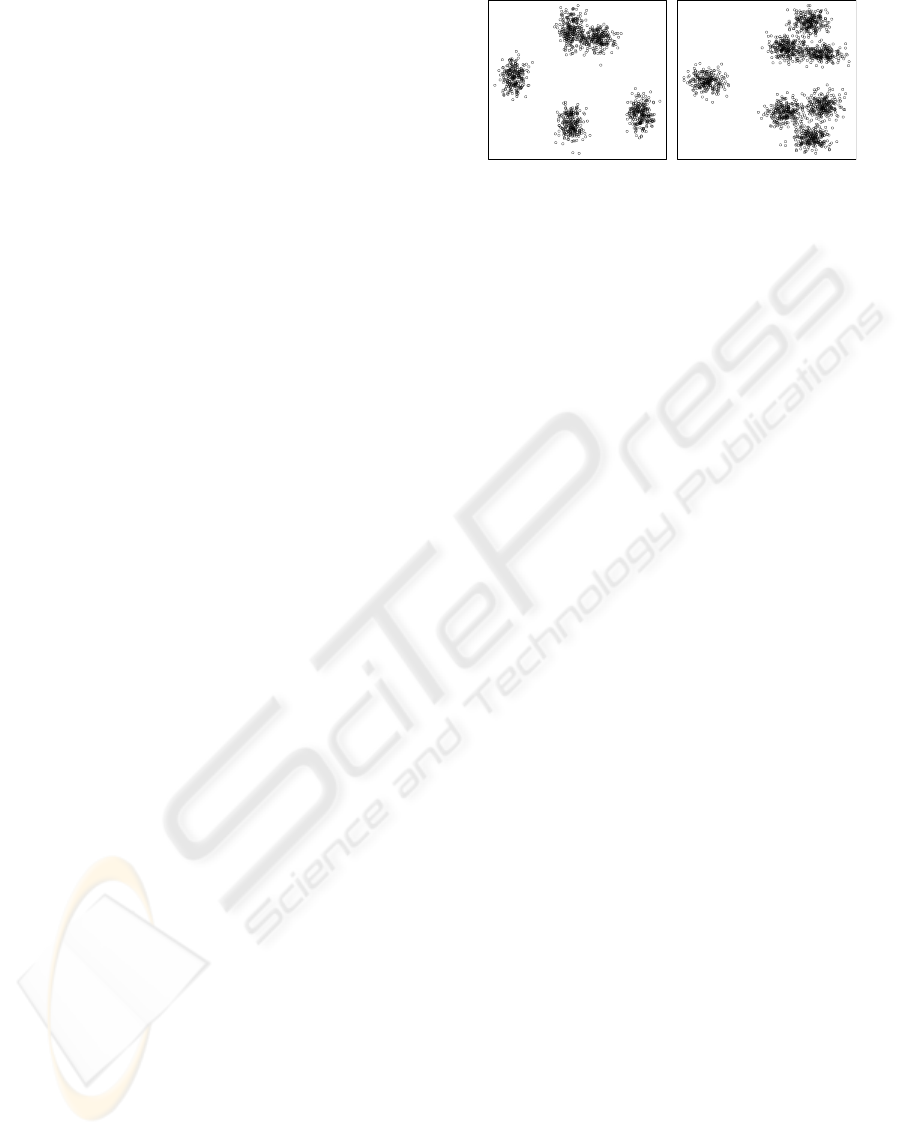
(a) (b)
Figure 1: Mixture of Gaussians data-sets. 1(a): Five Gaus-
sians, 1(b), seven Gaussians.
Mixtures of Gaussians. These data sets comprise
two mixtures of five and seven Gaussians with 1250
and 1750 points in two dimensions, respectively (Fig-
ure 1), where a certain number of overlappingpatterns
(potential ambiguities) can be observed. We used this
data sets with the purpose to provide an example of
the uncertainty problem in cluster ensembles.
Wine Data Set (WINE). The wine set is one of the
popular data sets from the UCI databank. It consists
of 178 instances with 13 attributes, representing three
different types of wines.
Wisconsin Breast Cancer Data Set (BREAST).
This data set constains 569 instances in 10 dimen-
sions, with 10 different features extracted from digi-
tised images of breast masses. The two existing
classes are referred to the possible breast cancer di-
agnosis (malignant, benign).
Handwritten Digits Data Set (PENDIG). The
third real data set is for pen-based recognition of
handwritten digits. In our experiments, we used the
test partition, composed of 3498 samples with 16 at-
tributes. Ten classes can be distinguished for the dig-
its 0-9.
3 CLUSTER ENSEMBLES
Diversifying Scenario. In order to achieve the re-
quired diversity of partitions in the ensemble, a ro-
bust centralised clustering scenario (RCC) has been
selected, using four different clustering methods: the
partition around medoids (pam), and the complete,
average and centroid linkage algorithms. Each clus-
tering method has been provided with the target num-
ber of clusters k, which is assumed to be known. Our
library or pool of clusterings is thus composed of four
component partitions, obtained by applying the four
mentioned clustering algorithms to the matrix of Eu-
clidean distances between the data objects. In the fol-
ICAART 2010 - 2nd International Conference on Agents and Artificial Intelligence
624

lowing, we refer to the clustering algorithms applied
to the raw Euclidean dissimilarities as base clusterers.
Consensus Function. A CSPA consensus function
has been applied to the ensemble partitions in order
to compute an aggregate cluster solution. Fist, the
CSPA algorithm derives the co-association matrix, A ,
whose elements A
ij
denote the number of times that
the objects i and j in the dataset have been assigned
to the same cluster by any pair of base clusterers in
the ensemble. As for the final consensus clustering,
a comparative analysis has been performed by apply-
ing again any of the aforementioned clustering meth-
ods, initially used as based clusterers, to cluster the
co-association matrix. At this stage, the clustering
algorithms are refered to as consensus clusterers, in
order to be distinguished from their respective previ-
ous roles as base clusterers. The decision for a unique
consensus clustering has not been addressed in this
paper. However, one option would be to use a supra
consensus by selecting the clustering with highest av-
erage normalised mutual information (ANMI), in a
similar way as suggested in (Strehl et al., 2002) for
choosing between different consensus heuristics.
Because the agglomerative and pam clustering al-
gorithms used in this work are based on dissimilarity
functions and the co-association matrix naturally rep-
resents similarities between objects, a conversion of
the co-association values has been performed as fol-
lows:
A
′
ij
= 1 −
A
ij
max(A )
(1)
so that the new co-association values A
′
denote
distances between the objects.
4 DETECTION OF AMBIGUOUS
REGIONS
In this section, we describe the approach used to de-
tect uncertain regions in a data set given the com-
ponent partitions in the ensemble. First, we need to
quantify the “uncertainness” of each data point. As
explained in Section 1, we assume ambiguous pat-
terns should lead to a lower consensus between the
ensemble partitions. Thus, the first goal is to measure
the agreement on which a given pattern is consistently
placed into the same cluster by the different base clus-
terers in the ensemble. The solution to this prob-
lem is not straightforward, given that the labels ren-
dered by a clustering algorithm are virtual labels and
cannot be directly compared. We propose a solution
based on the concept of mutual information (Cover
and Thomas, 1991) between different partitions. The
normalised mutual information (NMI) was proposed
in (Strehl et al., 2002) as a measure of the consensus
between two cluster solutions, λ
(a)
and λ
(b)
, (Equa-
tion 2).
NMI(λ
(a)
, λ
(b)
) = (2)
=
∑
k(a)
h=1
∑
k(b)
l=1
n
h,l
log
n·n
h,l
n
(a)
h
n
(b)
l
r
∑
k(a)
h=1
n
(a)
h
log
n
(a)
h
n
∑
k(b)
l=1
n
(b)
l
log
n
(b)
l
n
Denoting n, the number of observations in the
dataset, k(a) and k(b), the number of clusters in the
partitions λ
(a)
and λ
(b)
; n
(a)
h
and n
(b)
l
, the number of
elements in the clusters C
h
andC
l
of the partitions λ
(a)
and λ
(b)
respectively, and n
h,l
, the number of overlap-
ping elements between the clusters C
h
and C
l
.
For the present task, we measure the degree of
overlap between the clusters C
(a)
h
and C
(b)
l
containing
a pattern p under evaluation in the partitions λ
(a)
and
λ
(b)
, respectively. We call this metric the Normalised
Cluster Overlap (NCO):
NCO(λ
(a)
, λ
(b)
, p) =
n
h,l
r
n
(a)
h
log
n
(a)
h
n
n
(b)
l
log
n
(b)
l
n
(3)
The overall agreement in clustering the pattern is
then defined as the accumulated sum of NCOs con-
sidering all possible pairs of cluster partitions in the
ensemble:
ANCO(λ, p) =
L−1
∑
r=1
L
∑
r
′
=r+1
NCO(λ
(r)
, λ
(r
′
)
, p) (4)
Because ANCO is a measure of consensus, low
values correspond to patterns with higher uncertainty
and vice-versa.
Figure 3 shows an example of the patterns iden-
tified as ambiguities (in red colour) using the above
described approach on the mixtures of Gaussians.
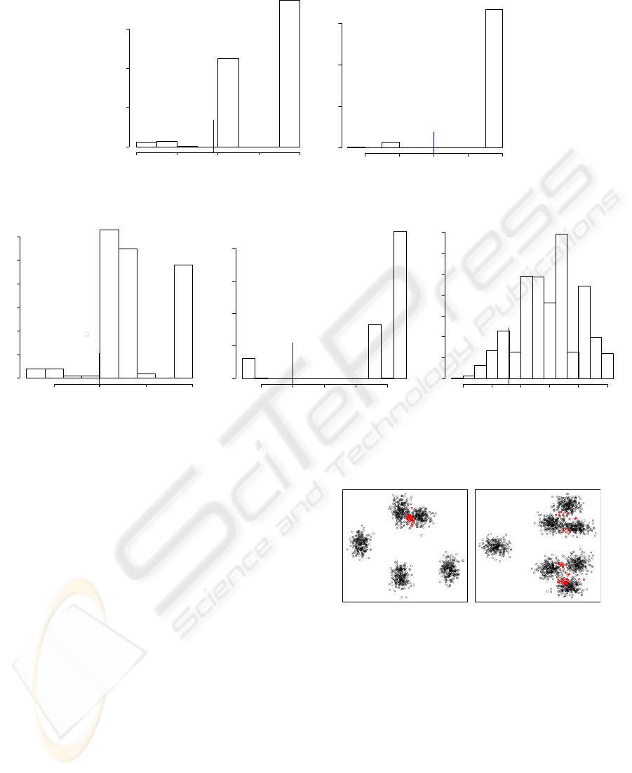
Finally, an ambiguous pattern is detected if its
ANCO value is found below a given threshold
ANCO
th
. In this work, the threshold value has been
determined by visualising the histogram plot of the
ANCO values. Figure 2 shows the histograms of
ANCO values in the analysed data sets and illustrates
the criterion for selecting the ANCO thresholds corre-
sponding to ambiguities. (Future work is to automate
this step).
ON AMBIGUITY DETECTION AND POSTPROCESSING SCHEMES USING CLUSTER ENSEMBLES
625
Histogram of ANCO values (FIVE GAUSSIANS)
ANCO values
Frequency
2 3 4 5 6
0
200
400
600
ANCOth=3.9
(a)
Histogram of ANCO values (SEVEN GAUSSIANS)
ANCO values
Frequency
2 3 4 5 6
0
500
1000
1500
ANCOth=4.0
(b)
Histogram of ANCO values (WINE)
ANCO values
Frequency
0.5 1.0 1.5 2.0
0
10
20
30
40
50
60
ANCOth=0.999
(c)
Histogram of ANCO values (BREAST)
ANCO values
Frequency
0.5 1.0 1.5 2.0 2.5
0
100
200
300
400
ANCOth=1.0
(d)
Histogram of ANCO values (PENDIG)
ANCO values
Frequency
0.0 0.5 1.0 1.5 2.0 2.5
0
100
200
300
400
500
600
700
ANCOth=0.8
(e)
Figure 2: Histogram plots used in the determination of the ANCO threshold in the evaluated data sets.
5 PROCESSING AMBIGUOUS
DATA
5.1 Support Vector Machines (SVM)
Support Vector Machines are amongst the most pop-
ular classification and regression algorithms because
of their robustness and good performance in com-
parison to other classifiers (Burges, 1998; Joachims,
1998; Lin et al., 2006). In its basic form, SVM were
defined for binary classification of linearly separa-
ble data. Let us denote a set of L training patterns
X = {x
1
, x
2
, ···x
L
} in R
D
. For binary classes, we
denote the set of labels corresponding to the training
data: Y = {y
1
, ··· , y
L
}, with y
i
∈ {1, −1} (Figure 4).
Assuming that the classes (+1,-1) are linearly sep-
arable, the SVM goal is to orientate a hyperplane
H which maximises the margin between the closest
members of the two classes (also called support vec-
tors). The searched hyperplane is given by the equa-
tion:
(a) (b)
Figure 3: Example of detected ambiguities in the mixtures
of Gaussians. Ambiguous patterns are depicted with red cir-
cles, in contrast to non-ambiguous patterns(black circles).
3(a): Five Gaussians, 3(b), seven Gaussians.
H := {x ∈ R
D
| wx+ b = 0} (5)
denoting w the normal vector of the hyperplane.
In addition, the parallel hyperplanes H
1
and H
2
at the
support vectors of classes y = 1 and y = −1 are de-
fined as:
H
1
:= {x ∈ R
D
| wx+ b = 1}, (y = 1)
H
2
:= {x ∈ R
D
| wx+ b = −1}, (y = −1) (6)
It can be demonstrated that the margin between
ICAART 2010 - 2nd International Conference on Agents and Artificial Intelligence
626
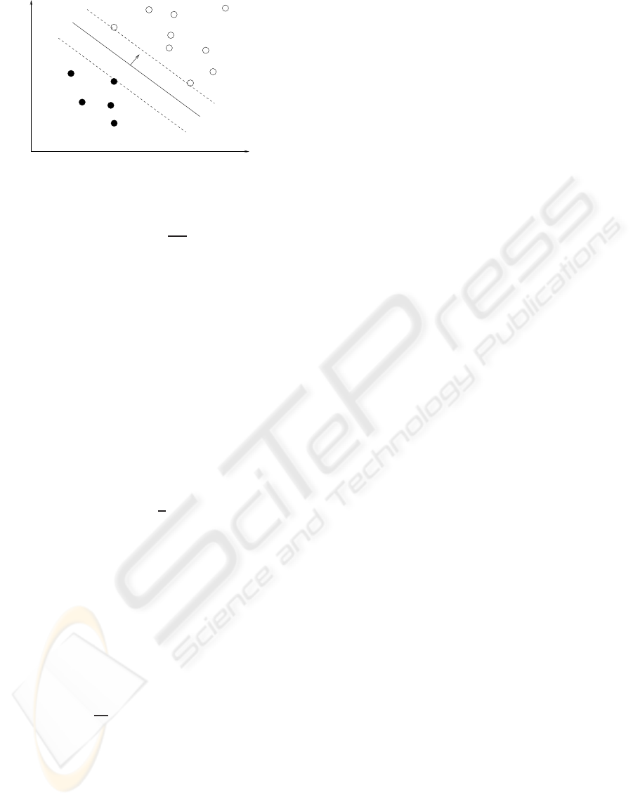
H2
H1
H
w
Figure 4: SVM example of binary classification through hy-
perplane separation (in this two-dimensional case the hyper-
plane becomes a line).
the hyperplanes H
1
and H
2
is
1
||w||
. In addition, the
training points at the left/right sides of the hyper-
planes H
1
and H
2
need to satisfy:
y
i
(wx
i
+ b) − 1 ≥ 0 ∀i (7)
Thus, the maximum margin hyperplane is ob-
tained by solving the following objective:
minimise k w k such that y
i
(wx+ b) − 1 ≥ 0 (8)
By applying Lagrange multipliers, the objective in
Equation 8 can be solved using constrained quadratic
optimisation. After some manipulations, it can be
shown that the initial objective is equivalent to:
maximise
L
∑
i=1
α
i
−
1
2
∑
j
α
i
α
j
y
i
y
j
x
i
x
j
subject to α
i
≥ 0 ∀i, and
L
∑
i=1
α
i
y
i
= 0 (9)
The solution of this quadratic optimisation prob-
lem is a set of coefficients α = {α
1
, ··· , α
L
} which are
finally applied to calculate the hyperplane variables w
and b:
w =
∑
α
i
y
i
x
i
b =
1
N
s
∑
s∈S
y
s
−
∑
m∈S
α
m
y
m
x
m
x
s
(10)
where S denotes the set of support vectors, of size
N
s
.
Although the solution in Equation 10 is found
for the basic problem of binary, linearly separable
classes, SVMs have been extended for both multi-
class and non-linear problems.
The Kernel Trick for Non-linearly Separable
Classes. The application of SVMs to non-linearly
separable classes is achieved by substituting the dot
product x
i
x
j
in Equation 8 by an appropriate function,
the so called kernel k(x
i
, x
j
). The purpose of this “ker-
nel trick” is that a non-linear kernel can be used to
transform the feature space into a new space of higher
dimension. In this high dimensional space it is pos-
sible to find a hyperplane to separate classes which
may not be originally separable in the initial space. In
other words, the kernel function is equivalent to the
dot product:
k(x
i
, x
j
) =< φ(x
i
)φ(x
j
) > (11)
where φ denotes a mapping of a pattern into the
higher dimensional space. The main advantage is that
the kernel computes these dot products without the
need to specify the mapping function φ.
Multi-class Classification. The extension for the
multi-class problem is achieved through a combi-
nation of multiple SVM classifiers. Two different
schemes have been proposed to solve this problem:
in a one-against-all approach, k hyperplanes are ob-
tained to separate each class from the rest of classes.
In a one-against-one approach, (
k
2
) binary classifiers
are trained to find all possible hyperplanes to separate
each pair of classes.
5.2 SVMs to Recluster Ambiguous Data
The simplest approach to deal with uncertainty is to
treat the ambiguous patterns as noise patterns and ig-
nore them, retaining the rest of data as good proto-
types for any further processing. However, reject-
ing uncertain data can result in a considerable loss of
relevant information, specially when these observa-
tions can help reveal the underlying data distribution.
Therefore, in this section we propose an alternative to
the simple rejection of the detected ambiguities based
on support vector machines.
First, patterns detected as ambiguous (Section 4)
are removed from the ensemble partitions. The co-
association matrix is then recalculated considering
only the unambiguous patterns. Intuitively, the re-
calculated co-association matrix should reflect higher
consensus among the combined partitions, as the re-
moved ambiguous patterns induced a certain “noise”
in this matrix. The consensus clustering is then ap-
plied to the new co-association matrix in order to
achieve a more robust aggregate solution. If no fur-
ther post-processing of the removed ambiguities is
performed, the described procedure up to this stage
corresponds to the simple removal of ambiguities.
Processing of Ambiguities. Now, we consider the
consensus solution obtained by using any of the afore-
mentioned clustering algorithms to recluster the new
ON AMBIGUITY DETECTION AND POSTPROCESSING SCHEMES USING CLUSTER ENSEMBLES
627

co-association matrix after removal of ambiguities.
Since this solution is achieved in absence of ambigu-
ous patterns, we assume a more robust representation
of the surrogate classes is attained in the output clus-
ters. Of course, a certain error is made by the cluster-
ing process, which can be measured if reference class
labels are available for a dataset, by calculating the
normalised mutual information (NMI) between the
cluster solution and the reference labels. However,
we ignore this error, assuming that the class structure
is adequately covered in the cluster solution. Next,
we assign a different “virtual” label to each one of
the obtained clusters - or classes. Thereby, a training
set is implicitely generated in an unsupervised man-
ner, using only the information in the ensemble - the
only supervised action involved in the whole process
is the selection of an ANCO threshold for detecting
ambiguous patterns, but we have shown (Section 4)
how this threshold can be easily determined by us-
ing histograms. This automatically generated train-
ing set is then used to train a model based on Support
Vector Machines to find the hyperplanes separating
the (virtual) classes. Finally, the SVM model is ap-
plied to make predictions on the ambiguous patterns,
previously removed from the ensemble. Hence, the
SVM decides which cluster in the consensus solution
an ambiguous pattern should be reallocated to.
6 EVALUATION AND TESTS
For evaluation purposes, we compared the clustering
solutions with the reference category labels, which
are available for all analysed data sets. There are dif-
ferent external validation metrics which can be used
to measure the correspondence between a cluster par-
tition and the reference labels, including entropy, pu-
rity (Boley et al., 1999), or the Normalised Mutual
Information (NMI, Equation 2). In this paper we se-
lected the latter one due to its property of impartiality
versus the number of clusters, in contrast to entropyor
purity, as suggested by Stern and Gosh (Strehl et al.,
2002).
We thus compared the NMI-based quality of the
ensemble consensus solutions (by using the agglom-
erative and pam algorithms as different consensus
clusterers applied to the co-association matrix) with
the values obtained by their respective base clusterers.
In addition, as is the focus of this work, we also eval-
uated the final ensemble solution when our scheme to
tackle ambiguities is introduced. In this respect, two
situations have been considered: (a) simple removal
of ambiguous patterns (in which case the category la-
bels corresponding to ambiguities have been also re-
moved from the reference label sets prior to test), and
(b) post-processing ambiguities with the help of sup-
port vector machines.
Tables 1 to 5 show the results obtained with the
evaluated approaches on the mixtures of Gaussians,
PENDIG, BREAST and WINE data sets. The first
rows show NMI values obtained by the base clusterers
(the complete, average and centroid linkages and the
partitioning around medoids applied on the original
matrix of object distances (ensemble components).
The second rowsrefer to the aggregate ensemble solu-
tions obtained by applying again the initial clustering
algorithms (complete, average, centroid linkage and
pam) as different consensus clusterers used to reclus-
ter the co-association matrices. The third rows indi-
cate the performance of the ensembles when the am-
biguity detection (AD) schemes are applied and the
ambiguous patterns are removed prior to consensus
clustering. Finally, the fourth and last rows show the
NMI values obtained by the final ensemble solutions
when the AD is introduced to detect ambiguities and
Support Vector Machines models are applied to post-
process and reallocate ambiguous data, using radial
and linear kernel functions (referred to as svm R and
L, respectively). Note also that the last columns in
each row refer to the average NMI scores of the four
clustering algorithms in each case.
As it can be observed, the ensemble approach out-
performs the corresponding base clusterers in all data
sets except WINE. The poorer performance in this
dataset can be associated to the inability of two of the
base clusterers (50% of the ensemble components) in
recovering any class structure (NMI values lower than
0.40%). This considerable proportion (50% of the en-
semble components) of “bad” clusterings has an im-
pact on the new co-association matrix, in such a way
that a third agglomerative approach fails to achieve an
adequate consensus, although the same algorithm was
originally able to recover more than 50% of the class
structure (NMI score) by using the object distance
matrix. On the other hand, note that the consensus
based on the partitioning around medoids algorithm
(pam) outperforms the corresponding base clusterer
in the ensemble (pam applied to original distances),
which also shows the best performance among the
base clusterers.
Nevertheless, the ensemble solutions outperform
the base components in all other data sets, where at
least 3/4 of the ensemble components are able to de-
tect some class structure (NMI values greater than
50%). The robustness of the ensemble solution is
also revealed by smaller standard deviations of NMI
scores across different consensus clusterings, in com-
parison to the respective base clusterings.
ICAART 2010 - 2nd International Conference on Agents and Artificial Intelligence
628

Table 1: Seven Gaussians data set.
Clustering
Avg.
comp. avg. cent. Pam
Base 0.907 0.913 0.915 0.945 0.920
Ensemble(E) 0.924 0.921 0.924 0.921 0.922
E + AD(ignore) 0.956 0.956 0.956 0.956 0.956
E + AD(svm L) 0.939 0.939 0.939 0.939 0.939
E + AD(svm R) 0.938 0.938 0.938 0.938 0.938
Table 2: Five Gaussians data set.
Clustering
Avg.
comp. avg. cent. Pam
Base 0.955 0.932 0.908 0.943 0.935
Ensemble (E) 0.943 0.945 0.945 0.945 0.944
E + AD(ignore) 0.974 0.974 0.974 0.974 0.974
E. + AD(svm L) 0.950 0.950 0.950 0.950 0.950
E. + AD(svm R) 0.949 0.949 0.949 0.949 0.949
Table 3: PENDIG data set.
Clustering
Avg.
comp. avg. cent. Pam
Base 0.537 0.652 0.030 0.658 0.469
Ensemble (E) 0.324 0.617 0.331 0.679 0.488
E + AD(ignore) 0.544 0.673 0.562 0.730 0.627
E + AD(svm L) 0.507 0.632 0.517 0.690 0.587
E + AD(svm R) 0.512 0.638 0.529 0.692 0.593
The incorporation of our approach to deal with
ambiguities shows important improvements with re-
spect to the standard ensemble. The best performance
is attained by detecting and rejecting ambiguous pat-
terns. The average increment of NMI scores ranges
from only one percentual point in the WINE dataset,
to 8% or 13.9% in the BREAST and PENDIG data
sets.
Also the reallocation of ambiguities using support
vector machines results in higher NMI scores when
compared to the initial ensemble. Different average
improvements are observed, up to 4.3% and 10.5% in
the BREAST and PENDIG data sets, respectively.
7 CONCLUSIONS AND FUTURE
DIRECTIONS
In this paper we have explored the cluster ensemble
problem, which aims at combining different cluster
partitions in order to improve the performance and
robustness of the aggregate solutions in comparison
to the ensemble components. In particular, we fo-
cused on the Cluster Similarity Partitioning scenario
(CSPA). This approach to cluster ensembles is to
combine the clusterings by calculating an intermedi-
Table 4: BREAST data set.
Clustering
Avg.
comp. avg. cent. Pam
Base 0.520 0.677 0.018 0.741 0.489
Ensemble (E) 0.685 0.685 0.685 0.685 0.685
E + AD(ignore) 0.766 0.766 0.766 0.766 0.766
E + AD(svm L) 0.726 0.726 0.726 0.726 0.726
E + AD(svm R) 0.728 0.728 0.728 0.728 0.728
Table 5: WINE data set.
Clustering
Avg.
comp. avg. cent. Pam
Base 0.550 0.031 0.038 0.721 0.335
Ensemble (E) 0.031 0.031 0.031 0.729 0.205
E + AD(ignore) 0.039 0.039 0.039 0.745 0.215
E + AD(svm L) 0.038 0.038 0.038 0.737 0.213
E + AD(svm R) 0.038 0.038 0.038 0.737 0.213
ate co-association matrix, which encodes the consen-
sus or agreement between the partitions in the ensem-
ble. The co-association matrix is used by any clus-
tering algorithm to provide a higher-level, consensus
clustering of the input data.
We further incorporate a strategy that is able to
detect ambiguous regions in the data by analysing
the different partitions in the ensemble. Prior to the
consensus clustering, the ambiguities detected are re-
moved from the component partitions, resulting in no-
table improvementsof the aggregatesolutions in com-
parison to the standard ensemble. We also propose
an approach to reallocate an ambiguous pattern into
one of the output clusters by using support vector ma-
chines in an unsupervised manner. An improvement
of the ensemble performance has also been observed
in this case.
Future work is to increase the number of clus-
terers in the ensemble and investigate ensemble se-
lection approaches (Fern and Lin, 2008) in order to
avoid the potential degradation of the ensemble per-
formance if a significant number of “bad” clusterers,
inappropriate for a dataset, are present among the en-
semble components.
REFERENCES
Boley, D., Gini, M., Gross, R., Han, E.-H., Karypis, G.,
Kumar, V., Mobasher, B., Moore, J., and Hastings, K.
(1999). Partitioning-based clustering for web docu-
ment categorization. Decis. Support Syst., 27(3):329–
341.
Burges, C. J. C. (1998). A tutorial on support vector
machines for pattern recognition. Data Mining and
Knowledge Discovery, 2:121–167.
ON AMBIGUITY DETECTION AND POSTPROCESSING SCHEMES USING CLUSTER ENSEMBLES
629

Cover, T. M. and Thomas, J. A. (1991). Elements of Infor-
mation Theory. John Wiley & sons.
Fern, X. Z. and Lin, W. (2008). Cluster ensemble selection.
In Proceedings of the SIAM International Conference
on Data Mining, pages 787–797.
Joachims, T. (1998). Text categorization with support vec-
tor machines: learning with many relevant features. In
Proceedings of ECML-98, 10th European Conference
on Machine Learning, number 1398, pages 137–142.
Kuncheva, L. I. (2004). Classifier ensembles for changing
environments. In Multiple Classifier Systems, pages
1–15. Springer.
Lin, Y.-M., Wang, X., Ng, W., Chang, Q., Yeung, D., and
Wang, X.-L. (2006). Sphere classification for ambigu-
ous data. In Proceedings of International Conference
on Machine Learning and Cybernetics, pages 2571–
2574.
Schapire, R. E. (2002). The boosting approach to machine
learning: An overview. In Proceedings of the 2002
MSRI Workshop on Nonlinear Estimation and Classi-
fication, pages 149–173. Springer.
Strehl, A., Ghosh, J., and Cardie, C. (2002). Cluster en-
sembles - a knowledge reuse framework for combin-
ing multiple partitions. Journal of Machine Learning
Research, 3:583–617.
ICAART 2010 - 2nd International Conference on Agents and Artificial Intelligence
630
