A NON-PARAMETERISED HIERARCHICAL POLE-BASED
CLUSTERING ALGORITHM (HPOBC)
Amparo Albalate, Steffen Rhinow
Institute of Information Technology, University of Ulm, Ulm, Germany
David Suendermann
SpeechCycle Labs, NY, U.S.A.
Keywords:
Divisive clustering, PoBOC, Silhouette width.
Abstract:
In this paper we propose a hierarchical, divisive, clustering algorithm, called Hierarchical Pole Based Clus-
tering (HPoBC), which is able to find the clusters in a data set without any user input parameter such as the
number of clusters k. The algorithm is based on the Pole Based Overlapping Clustering (PoBOC) (Cleuziou
et al., 2004). Initially, the top hierarchy level is composed by the set of clusters discovered by the PoBOC
algorithm on the dataset. Then, each single cluster is again analysed using a combination of PoBOC and clus-
ter validity methods (silhouettes) in order to search for new possible subclusters. This process is recursively
repeated on each newly retrieved cluster until the silhouette score suggests to stop any further partitioning
of the cluster. The HPoBC algorithm has been compared to the original PoBOC as well as other classical
hierarchical approaches on five two-dimensional, synthetic data sets, using three cluster evaluation metrics.
1 INTRODUCTION
Cluster analysis refers to techniques used to discover
the group structure in a certain data set. These al-
gorithms have multiple applications, such as image
segmentation, text mining, or the analysis of genomic
and sensorial data, among others.
A large variety of clustering techniques have been
proposed over the past decades. Because no prior
knowledge is required about the object’s group labels,
clustering algorithms are unsupervised learning mod-
els. However, most algorithms in the clustering lit-
erature are parameterised approaches, i.e, the cluster
solutions depend on some user input parameters de-
scriptive for the dataset. Typical input parameters are
the target number of clusters, or density indicators in
density models.
The Pole-Based OverlappingClustering algorithm
(PoBOC), proposed in (Cleuziou et al., 2004), is an
overlapping, graph-based clustering approach which
does not require any input information from the user.
The algorithm iteratively identifies a set of initial clus-
ter prototypes, and builds the clusters around these
objects based on the objects’ neighbourhoods.
One limitation of the PoBOC algorithm is related
to the neighbourhood formulation applied to extract
the final clusters. The neighboorhood of one object
is defined in terms of the object’s average distance to
all other objects in the data set (see Section 2.1). This
global definition can be suitable for discovering uni-
formly spread clusters on the data space. However,
the algorithm may fail to identify all existing clusters
if the input data is organised in a hierarchy of classes,
in such a way that two or more subclasses are closer
to each other than the average class distance.
In order to overcome this limitation, we propose
a new hierarchical algorithm based on PoBOC, called
“Hierarchical Pole-Based Clustering” (HPoBC). The
hierarchy of clusters and subclusters is detected
though a recursive approach. First, the PoBOC al-
gorithm is used to identify the clusters in the data set,
also referred to as “poles”. Next, under the hypoth-
esis that more subclusters may exist inside any pole,
PoBOC is again locally applied to each initial pole. A
cluster validity based on silhouette widths is then used
in order to validate or reject the subcluster hypothesis.
If the subcluster hypothesis is rejected by the silhou-
ette score, we discard the candidate subclusters and
select the initial pole as part of the output clusters.
Otherwise (the hypothesis is validated) we store the
350
Albalate A., Rhinow S. and Suendermann D. (2010).
A NON-PARAMETERISED HIERARCHICAL POLE-BASED CLUSTERING ALGORITHM (HPOBC).
In Proceedings of the 2nd International Conference on Agents and Artificial Intelligence - Artificial Intelligence, pages 350-356
DOI: 10.5220/0002735003500356
Copyright
c
 SciTePress

new identified poles (subclusters) and continue with a
similar analysis inside each new pole. This procedure
is applied recursively until the silhouette rejects every
further hypothesis.
The paper is organised as follows: In Section 2
an overview of the PoBOC algorithm is presented. In
Section 3, we introduce some of the classical hierar-
chical clustering approaches. In Section 4, the new
HPoBC algorithm is described in detail. Finally, in
Sections 5 and 6, we present evaluation results and
draw conclusions, respectively.
2 THE POLE-BASED
OVERLAPPING CLUSTERING
(PoBOC)
The Pole-Based Overlapping Clustering is an overlap-
ping, graph-based clustering technique proposed by
(Cleuziou et al., 2004). The algorithm takes the ma-
trix of object dissimilarities as single input and builts
the output clusters in four main steps: (i) Definition
of dissimilarity graph, (ii) construction of poles, (iii)
pole restriction and (iv) affectation of objects to poles.
2.1 Definition of a Dissimilarity Ggraph
Let X denote the set of n data points (objects) in the
data set, and D the dissimilarity matrix, computed
over X .
The dissimilarity graph G⊲X ,V, D⊳ is then spec-
ified by: (i) the dissimilarity matrix D, (ii) the data
points or vertices, X , and a set of edges V between
all pairs of vertices ⊲x
i
, x
j
⊳ corresponding to mutual
neighbour points.
Definition 1. (Neighbourhood of a point x): The
neighbourhood of a point x, denoted by N⊲x⊳ is com-
posed of all points of X whose dissimilarity to the
point is smaller than the mean distance of the object x
to all other objects in X (d
mean
⊲xI X ⊳):
N⊲x⊳ D {x
j
∈ X |D
x
j
,x
< d
mean
⊲xI X ⊳} (1)
Definition 2. Two points ⊲x
i
, x
j
⊳ are mutual neigh-
bours, and thus connected by an edge in the Graph G
if each one belongs to the neighbourhood of the other:
⊲x
i
, x
j
⊳ ∈ V ↔ x
i
∈ N⊲x
j
⊳I x
j
∈ N⊲x
i
⊳ (2)
2.2 Pole Construction
This procedure builds incrementally a set of poles
P D {P
1
, P
2
. . . , P
k
}, over X , based on the dissimilar-
ity matrix D and the dissimilarity graph G⊲X ,V, D⊳.
Let O denote the cumulated set of objects that belong
to any of the extracted poles up to the current state
(initially the empty set).
The poles are grown from initial points
O
x
i
, which
are the points with maximum mean distance to the
cumulated set of poles O. Initially, the object
O
x
0
with
maximum distance to X is selected:
O
x
0
D argmax
x∈X
⊲d
mean
⊲x, X ⊳⊳ (3)
O
x
i
D argmax
x∈X \O
⊲d
mean
⊲x, O⊳⊳ (4)
Each P
i
pole is then grown from the corresponding
initial object
O
x
i
, in such a way that all the pole mem-
bers are enclosed in their respective neighbourhoods.
This is implemented in the build-pole procedure:
Algorithm 1. Build-pole (
O
x, G⊲X ,V, D⊳).
Input: initial point
O
x, dissimilarity graph G⊲X ,V, D⊳
Output: pole built around
O
x, P
Initialise: P D
O
x
Obtain neighbourhood of P:
N⊲P⊳ D {x ∈ X |∀x
i
∈ P, ⊲x,x
i
⊳ ∈ V}
while N⊲P⊳ 6D
/
0 do
attach the object x to P such that:
x ∈ N⊲P⊳ and x D argmax
x
i
∈N⊲P⊳
d
mean
⊲x
i
, P⊳
Update N⊲P⊳
end while
Return P
The selection of the initial object
O
x
i
and the con-
struction of the corresponding pole P
i
is iteratively re-
peated until all objects in the data set are contained
in any of the poles, O D X , or no initial object can
be found which is sufficiently distant from the set of
poles.
2.3 Pole Restriction
After the pole construction, overlapping objects may
be obtained, which simultaneously belong to the
neighbourhood of two or more poles. These objects
compose the residual set R. The pole restriction pro-
cedure consists of removing residual objects from the
original poles, resulting in a new set of reduced, non-
overlapping poles
Q
P.
2.4 Affectation Stage
The set of residual objects R obtained at the pole re-
striction stage require some post-processing strategy,
in order to be reallocated into one or more of the re-
stricted poles. This reallocation of objects in PoBOC
is called affectation. First, the membership of each
object x to each
Q
P
i
restricted pole, u⊲x,
Q
P
i
⊳ is com-
puted as:
A NON-PARAMETERISED HIERARCHICAL POLE-BASED CLUSTERING ALGORITHM (HPOBC)
351

u⊲x,
Q
P
i
⊳ D 1−
d
mean
⊲x,
Q
P
i
⊳
D
max
(5)
Next, the objects are affected to one or more
poles. In a single-affectation approach, each object
x is assigned to the pole maximising the membership
u⊲x,
Q
P
j
⊳. In a multi-affectation approach, the object is
affected to the poles whose memberships are greater
than some reference values given by a linear approx-
imation on the set of object memberships, sorted in
decreasing order.
3 HIERARCHICAL CLUSTERING
Classical approaches for hierarchical clustering ob-
tain the cluster solution by iterative mergings or di-
visions of clusters (Everitt, 1974; Kaufmann and
Rousseeuw, 1990). Two major hierarchical ap-
proaches can be distinguished: agglomerative and di-
visive.
Hierarchical Agglomerative Approaches. Ag-
glomerative algorithms are the so-called bottom-up
approaches, starting with all points as individual
clusters and successively merging the closest pair
of clusters until all patterns are enclosed in a single
cluster. The algorithms can be visualised using a
graphical tree structure called dendogram where
the pair of clusters that are merged at each iteration
can be observed. The final cluster solution is se-
lected by the user, by specifying a level to cut the
dendogram or, equivalently, a desired number k of
clusters. Different agglomerative approaches can be
distinguished, depending on the proximity criterion
to merge the next pair of clusters. For example,
while the single linkage algorithm selects the pair of
clusters with the minimum distance between their
closest elements, the complete linkage algorithm
selects the clusters with minimum distance between
the farthest objects. In a similar way, the average
linkage and centroid algorithms choose the clusters
with the minimum average inter cluster distance and
the minimum distance between their centroid objects,
respectively.
Hierarchical Divisive Approaches. As opposed to
agglomerative algorithms, a divisive approach, such
as the divisive analysis (DiANA) algorithm, starts at
the top dendogram level where all objects compound
a unique cluster and iteratively splits the biggest clus-
ter until each object is in its own cluster. The reader is
referred to (Everitt, 1974) for more details about the
divisive analysis algorithm.
4 NEW HIERARCHICAL
POLE-BASED APPROACH
The new clustering method is combination of the
PoBOC algorithm and hierarchical divisive clustering
strategies. In a divisive manner, the proposed hier-
archical approach is initialised with the set of poles
identified by the PoBOC algorithm, and recursively
applied to each obtained pole, searching for possible
subclusters.
4.1 Pole-based Clustering Basis Module
In order to detect the set of poles in the new hierarchi-
cal approach, the graph construction, pole construc-
tion and pole restriction stages of POBOC have been
preserved, but the affectation step has been replaced
by a new procedure called pole regrowth:
Algorithm 2. Pole regrowth (
Q
P, R, D).
Input: sets of poles and residual from the pole-reduction
step:
Q
P, R; dissimilarity matrix D
Output: set of regrown poles
O
P
Initialise:
O
P D
Q
P
while R 6D
/
0 do
Find the pair (x
i
∈ R,
O
P
j
∈
O
P) with minimum distance:
⊲x
i
,
O
P
j
⊳ D argmin
x∈R,
O
P∈
O
P
D
min
⊲x,
O
P⊳,
with D
min
⊲x
i
,
O
P
j
⊳ D min
x
k
∈
O
P
j
D
ik
Attach the point x
i
to its closest pole and remove it
from the residual set:
O
P
j
D
O
P
j
∪ x
i
R D R − x
i
end while
Return
O
P
The pole-regrowth procedure is an alternative to
the PoBOC single affectation for reallocating overlap-
ping objects into one of the restricted poles. As it can
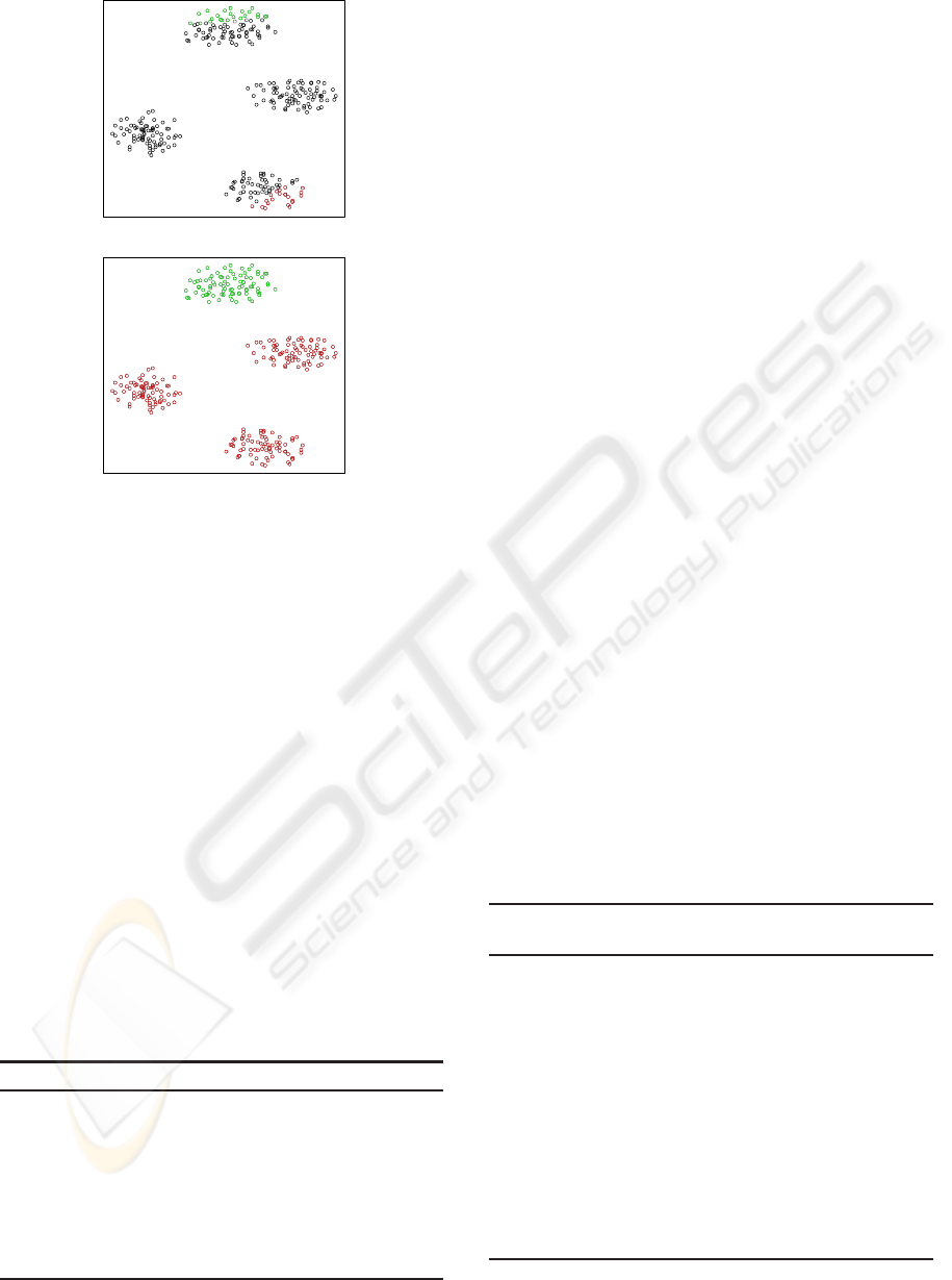
be observed in Figure 1(a), not only a pole but also an
overlapping region may contain potential subclusters.
If each overlapping object x
i
is individually assigned
to the pole maximising the membership u⊲x
i
I
Q
P⊳, the
objects inside a single cluster might be assigned to
different poles
1
. The pole regrowth procedure is in-
tended to avoid any undesired partitioning of clusters
existing in overlapping areas while reallocating resid-
ual objects.
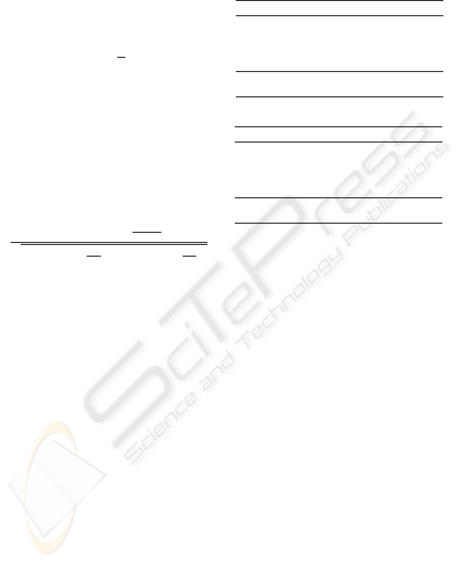
An example of the pole regrowth method is shown
in Figure 1. Figure 1(a) shows two restricted poles
1
Note that the hierarchical approach is independently
applied to the grown poles.
ICAART 2010 - 2nd International Conference on Agents and Artificial Intelligence
352

(a)
(b)
Figure 1: Example of the pole growth.1(a) Two restricted
poles (red and green circles) and their overlapping objects
(black circles) - from the database 1000p9c. 1(b) New poles
obtained after the reallocation of overlapping objects by the
pole regrowth method.
in red and green colours, respectively. All points be-
tween these restricted poles are overlapping points. It
can be observed that many of these overlappingpoints
build another two clusters, which PoBOC fails to de-
tect. The reallocation of overlapping points by the
pole regrowth procedure is illustrated in Figure 1(b).
A single affectation would have splitted each overlap-
ping cluster in two halfs (upper and bottom). Using
the pole regrowth, all objects inside each overlapping
cluster have been jointly assigned into a single pole.
This fact allows to detect the overlapping clusters in
further recursive steps.
We refer to the modified PoBOC algorithm as
Pole-Based clustering module, which is the basis for
the hierarchical approach described in the following
paragraphs:
Algorithm 3. Pole-based clustering module (X ).
Input: set of data points to be clustered X
Output: set of regrown poles
O
P
Compute dissimilarity matrix of X : D
Compute dissimilarity graph over X , G⊲X ,V, D⊳
P ← Pole Construction (X , D, G⊲X ,V, D⊳)
Q
P, R ← Pole Restriction (P)
O
P ← Pole Regrow (
Q
P, R, D)
Return
O
P.
4.2 Hierarchical Pole-based Clustering
(HPoBC)
The proposed algorithm is called Hierarchical Pole-
Based Clustering (HPoBC).
First, the Pole-Based Clustering module is applied
to the entire dataset to obtain an initial set of poles.
Then, a recursive function, the Pole-Based Subclus-
ter Analysis is triggered on each pole with more than
one object. If an individual pole is found, the cor-
responding object is attached to the set of final clus-
ters as an individual cluster. This recursive function
is continuously called with the objects of each ob-
tained pole, internally denoted
O
P
top
, because it refers
to an upper level in the hierarchy. Analogously, the
new set of poles found on
O
P
top
is denoted
O
P
sub
, in-
dicating a lower hierarchy level. These poles repre-
sent candidate subclusters. In order to decide wether
O
P
sub
compounds “true” subclusters or not, a criterion
typically used for cluster validity is applied, namely
the average silhouette width (Rousseeuw, 1987). The
silhouette width of a cluster partition returns a qual-
ity score in the range [-1,1] where 1 corresponds to
a perfect clustering. According to (Treeck, 2005), a
silhouette score smaller or equal than 0.25 is an indi-
cator for wrong cluster solutions. However, from our
experiments, a more rigorous threshold sil > 0.5 has
proven adequate for validating the candidate subclus-
ters. The problem of deciding whether a data set con-
tains a cluster structure or not is commonly referred
to as cluster tendency in the cluster literature (Jolion
and Rosenfeld, 1989). If the quality criterion is not
fulfilled ⊲sil < 0.5⊳ the subcluster hypothesis is re-
jected, and the top cluster
O
P
top
is attached to the final
clusters. Otherwise, we continue exploring each sub-
cluster in order to search for more possible sublevels.
Algorithm 4. Hierarchical Pole-Based Clustering -
HPoBC (X ).
Input: Set of data points to be clustered X
Output: A cluster partition of X : Clusters
Initialise: Clusters = {
/
0}
Obtain set of grown poles on all X objects:
O
P ← Pole-Based Clustering Module(X )
for all
O
P
i
∈
O
P do
if |
O
P
i
| > 1 then
Trigger recursive search for subclusters:
Pole-Based Subcluster Analysis (
O
P
i
, Clusters)
else
Add
O
P
i
to Clusters
end if
end for
Return Clusters
A NON-PARAMETERISED HIERARCHICAL POLE-BASED CLUSTERING ALGORITHM (HPOBC)
353

Algorithm 5. Pole-based Subcluster Analysis (
O
P
top
,
Clusters).
O
P
sub
← Pole-Based Clustering Module(
O
P
top
)
stop ← (silhouette-width⊲
O
P
sub
⊳ ≤ 0.5)
if stop=true then
Add
O
P
top
to Clusters
Return
else
for all
O
P
sub
i
∈
O
P
sub
do
if |
O
P
i
sub
| > 1 then
Pole-Based Subcluster Analysis (
O
P
sub
i
, Clusters)
else
Add
O
P
sub
i
to Clusters
Return
end if
end for
end if
5 EVALUATION METHODS
The PoBOC algorithm as well as the hierarchical
Pole-Based clustering (HPoBC) have been compared
to other hierarchical approaches: the single, com-
plete, centroid and average linkage and the divisive
analysis (DiANA) algorithm. These classical hier-
archical algorithms are examples of clustering ap-
proaches that require the target number of clusters (k)
in order to find the cluster solutions. In order to allow
for a comparison of PoBOC and HPoBC to the hier-
archical agglomerative approaches, these algorithms
have been called with different values of the k pa-
rameter, and the silhouette index has been applied to
validate each solution and predict the optimum num-
ber of clusters, k
opt
. Note that, while the Silhouette
index is used in agglomerative algorithms and Di-
ANA as a cluster validity strategy to select the opti-
mum k among a set of K possible cluster solutions, in
the hierarchical Pole-Based algorithm, the Silhouette
scores are applied in a recursive and “local” manner,
in order to evaluate the cluster tendency inside each
obtained pole.
Data Sets. The described approaches have been ap-
plied to the synthetic data sets of Figure 2: The first
dataset (100p5c) comprises 100 objects in 5 spatial
clusters (Figure 2 (a)), the second dataset (6Gauss) is
a mixture of six Gaussians (1500 points) in two di-
mensions (Figure 2(e)). The third data set (3Gauss)
is a mixture of three Gaussians (800 points) in which
the distance of the biggest class to the other two is
larger than the distance among the two smaller Gaus-
sians (Figure 2(i)). This data set illustrates a typical
example in which using cluster validity based on Sil-
houettes may fail to predict the number of classes due
to the different interclass distances. The fourth and
fifth data (560p8c and 1000p9c) contain 560 and 1000
points in two dimensions, with 8 and 9 spatial clus-
ters, respectively (Figures 2(m) and (q)).
The cluster solutions provided by PoBOC,
HPoBC and an example hierarchical agglomerative
approach (average linkage) are shown in the plots of
Figure 2 (different colours are used to indicate differ-
ent clusters).
5.1 Cluster Evaluation Metrics
For a comprehensive evaluation of the discussed al-
gorithms, their cluster solutions have been also com-
pared with the reference category labels, available
for evaluation purposes, using three typical external
cluster validation methods: Entropy, Purity, and Nor-
malised Mutual Information.
Entropy. The cluster entropy (Boley et al., 1999)
reflects the degree to which the clusters are composed
of heterogeneous patterns, ie, patterns that belong to
different categories. According to the Entropy crite-
rion, a good cluster should be mostly aligned to a sin-
gle class, which means that a large number of the clus-
ter objects belong to the same category. This quality
condition corresponds to low entropy values. The en-
tropy of a cluster i is defined as:
E
i
D −
L
∑
jD 1
p
ij
log
2
⊲p
ij
⊳ (6)
where L denotes the number of reference categories,
and p
ij
, the probability that an element of category j
is found in cluster i. This probability can be formu-
lated as p
ij
D
n
j
ni
, denoting n
j
the number of elements
of class j in the cluster i, and n
i
, the total number of
elements in the cluster i.
The total entropy of the cluster solution C is ob-
tained by averaging the cluster entropies according to
Equation 7 (n denotes the total number of elements in
the data set):
E⊲C⊳ D
k
∑
iD 1
n
i
n
E
i
(7)
As discussed above, “good” cluster solutions yield
small entropy values.
Purity. Like entropy, purity (Boley et al., 1999; Wu
et al., 2009) is a metric to measure the extent to which
a cluster contains elements of a single category. The
ICAART 2010 - 2nd International Conference on Agents and Artificial Intelligence
354

purity of a cluster i is defined in terms of the maxi-
mum class probability, P
i
D max
j
⊲p
ij
⊳
The overall purity of a cluster solution is calcu-
lated by averaging the cluster purities:
P⊲C⊳ D
k
∑
iD 1
n
i
n
P
i
(8)
Higher purity values indicate a better quality of
the clustering solution, up to a purity value equal to
one, which is attained when the cluster partition is
perfectly aligned to the reference classes.
Normalised Mutual Information (NMI). The
Normalised Mutual information (NMI) measures the
agreement between two partitions of the data, C
⊲a⊳
and C
⊲b⊳
, (Equation 9).
NMI⊲C
⊲a⊳
, C
⊲b⊳
⊳ D (9)
D
∑
k⊲a⊳
hD 1
∑
k⊲b⊳
lD 1
n
h,l
log

n·n
h,l
n
⊲a⊳
h
n
⊲
l
b⊳

q
⊲
∑
k⊲a⊳
hD 1
n
⊲a⊳
h
log

n
⊲a⊳
h
n

⊳⊲⊲
∑
k⊲b⊳
lD 1
n
⊲b⊳
l
log

n
⊲b⊳
l
n

⊳
Denoting n, the number of observations in the
dataset, k⊲a⊳ and k⊲b⊳, the number of clusters in the
partitions C
⊲a⊳
and C
⊲b⊳
; n
⊲a⊳
h
and n
⊲b⊳
l
, the number
of elements in the clusters C
h
and C
l
of the partitions
C
⊲a⊳
and C
⊲b⊳
, respectively, and n
h,l
, the number of
overlapping elements between the clusters C
h
and C
l
.
The normalised mutual information can be used as a
quality metric of a cluster partition by comparing the
cluster solution C with the reference class labels L,
NMI⊲C, L⊳.
5.2 Results
As can be seen in Tables 1 to 5, the performance of
the HPoBC algorithm is consistently superior to the
original PoBOC algorithm on all datasets and met-
rics. The classical (divisive and agglomerative) ap-
proaches with the help of Silhouettes to determine
the optimum k are also able to detect the class struc-
ture in three data sets (100p5c, 1000p9c and 6Gauss).
The performance of classical approaches is thus com-
parable to the HPoBC algorithm on the mentioned
data sets. Note that, in some cases, the NMI score
achieved by HPoBC is marginally inferior (≤ 1.8%)
to other hierarchical approaches, due to the false dis-
covery by HPoBC of tiny clusters in the boundaries
of a larger cluster. In contrast to the previous data
sets, the DiANA and agglomerative hierarchical ap-
proaches fail to capture accurately the existing classes
on the datasets 560p8c and 3Gauss. The problem lies
Table 1: 560p8c Data.
Clustering # Clusters NMI Purity Entropy
DiANA 5 0.850 0.660 0.840
single 5 0.850 0.660 0.840
complete 5 0.850 0.660 0.840
average 5 0.850 0.660 0.840
centroid 5 0.850 0.660 0.840
PoBOC 4 0.801 0.548 1.048
HPoBC 7 0.944 0.867 0.287
Table 2: 100p5c Data.
Clustering # Clusters NMI Purity Entropy
DiANA 5 1 1 0
single 5 1 1 0
complete 5 1 1 0
average 5 1 1 0
centroid 5 1 1 0
PoBOC 3 0.801 0.693 0.817
HPoBC 5 1 1 0
in the Silhouette scores, which fail to place the max-
imum (k
opt
) at the correct number of clusters. This
happens because the intra-class separation differs sig-
nificantly among the clusters. However, this problem
is not observed in the HPoBC algorithm, since Sil-
houette scores are used to evaluate the local cluster
tendency. This implies a more “relaxed” condition
in comparison to the use of Silhouettes for validating
global clustering solutions. Thus, in these cases, the
HPoBC algorithm is advantageous with respect to the
classical hierarchical approaches, as evidenced by ab-
solute NMI improvements around 10%.
5.3 Complexity Considerations for
Large Databases
If denoting n, the total number of objects in the data
set, the complexity of the PoBOC algorithm is es-
timated in the order of O⊲n
2
⊳, similar to the clas-
sical hierarchical schemes. The complexity of the
Pole-Based Hierarchical Clustering depends on fac-
tors such as the number and size of poles retrieved
at each step and the maximum number of recursive
steps necessary to obtain the final cluster solution.
The worst case in terms of the algorithm efficiency
would happen if a pole with n− 1 elements were con-
tinuously found until all elements composed individ-
ual clusters. In this case, the algorithm would reach
a cubic complexity O⊲n⊲n C 1⊳⊲2n C 1⊳⊳. In gen-
eral terms, if k is the number of recursive steps (lev-
els descended in the hierarchy) necessary to reach the
solution, the maximum complexity of the algorithm
can be approximated as O⊲k · n
2
⊳. As for the anal-
A NON-PARAMETERISED HIERARCHICAL POLE-BASED CLUSTERING ALGORITHM (HPOBC)
355

Table 3: Mixture of six Gaussians.
Clustering # Clusters NMI Purity Entropy
DiANA 6 0.980 0.992 0.049
single 6 1 1 0
complete 6 1 1 0
average 6 1 1 0
centroid 6 1 1 0
PoBOC 3 0.606 0.693 0.817
HPoBC 7 0.982 1 0
ysed datasets, the algorithm needed 3 recursive steps
at most to achieve the presented results. It leads to a
quadratic complexity, comparable to the PoBOC al-
gorithm and the rest of hierarchical approaches.
Table 4: 1000p9c.
Clustering # Clusters NMI Purity Entropy
DiANA 9 1 1 0
single 9 1 1 0
complete 9 1 1 0
average 9 1 1 0
centroid 9 1 1 0
PoBOC 5 0.837 0.634 0.637
HPoBC 11 0.993 1 0
Table 5: Mixture of 3 Gaussians.
Clustering # Clusters NMI Purity Entropy
DiANA 2 0.847 0.812 0.375
single 2 0.847 0.812 0.375
complete 2 0.847 0.812 0.375
average 2 0.847 0.812 0.375
centroid 2 0.847 0.812 0.375
PoBOC 2 0.847 0.812 0.375
HPoBC 4 0.990 1 0
6 CONCLUSIONS
In this paper we present a hierarchical clustering ap-
proach based on the Pole-Based Clustering algorithm
(PoBOC), which only needs the objects in a dataset
as input, in contrast to other approaches that require
the number of clusters as input parameter. The use of
global object distances by PoBOC does not allow to
differentiate between subclusters, specially if the data
is organised in a hierarchy. We therefore propose a
hierarchical version of PoBOC, called HPoBC, that
recursively applies into each obtained cluster in order
to adapt the object distances to local regions and accu-
rately retrieve clusters as well as subclusters. Results
obtained on five spatial databases have proventhe bet-
ter performance of the new hierarchical approach with
respect to the baseline PoBOC, also comparable or
superior with respect to other traditional hierarchical
approaches. However, we need to emphasize the fact
that the presented results have been obtained on syn-
thetic data sets with noticeable differences between
intercluster distances. In future work we further ex-
pect to validate the performance of the HPoBC algo-
rithm on real databases.
REFERENCES
Boley, D., Gini, M., Gross, R., Han, E.-H., Karypis, G.,
Kumar, V., Mobasher, B., Moore, J., and Hastings, K.
(1999). Partitioning-based clustering for web docu-
ment categorization. Decis. Support Syst., 27(3):329–
341.
Cleuziou, G., Martin, L., Clavier, L., and Vrain, C. (2004).
Poboc: An overlapping clustering algorithm, applica-
tion to rule-based classification and textual data. In
Proceedings of the 16th European Conference on Ar-
tificial Intelligence ECAI.
Everitt, B. (1974). Cluster Analysis. Heinemann Educ.,
London.
Jolion, J.-M. and Rosenfeld, A. (1989). Cluster detection in
background noise. Pattern Recogn., 22(5):603–607.
Kaufmann, L. and Rousseeuw, P. J. (1990). Finding Groups
in Data. An Introduction to Cluster Analysis. Wiley,
New York.
Rousseeuw, P. (1987). Silhouettes: A graphical aid to the
interpretation and validation of cluster analysis. Jor-
nal Comp. Appl. Math., 20:53–65.
Treeck, B. (2005). Entwicklung und Evaluierung einer
Java-Schnittstelle zur Clusteranalyse von Peer-to-
Peer Netzwerken. Bachelorarbeit. Heinrich-Heine-
Universit¨at D¨usseldorf.
Wu, J., Chen, J., Xiong, H., and Xie, M. (2009). Ex-
ternal validation measures for k-means clustering:
A data distribution perspective. Expert Syst. Appl.,
36(3):6050–6061.
ICAART 2010 - 2nd International Conference on Agents and Artificial Intelligence
356