ON THE GRADIENT-BASED ALGORITHM FOR MATRIX
FACTORIZATION APPLIED TO DIMENSIONALITY REDUCTION
Vladimir Nikulin and Geoffrey J. McLachlan
Department of Mathematics, University of Queensland, Brisbane, Australia
Keywords:
Matrix factorisation, Gradient-based optimisation, Cross-validation, Gene expression data.
Abstract:
The high dimensionality of microarray data, the expressions of thousands of genes in a much smaller number
of samples, presents challenges that affect the applicability of the analytical results. In principle, it would be
better to describe the data in terms of a small number of metagenes, derived as a result of matrix factorisation,
which could reduce noise while still capturing the essential features of the data. We propose a fast and general
method for matrix factorization which is based on decomposition by parts that can reduce the dimension
of expression data from thousands of genes to several factors. Unlike classification and regression, matrix
decomposition requires no response variable and thus falls into category of unsupervised learning methods.
We demonstrate the effectiveness of this approach to the supervised classification of gene expression data.
1 INTRODUCTION
The analysis of gene expression data using matrix fac-
torization has an important role to play in the discov-
ery, validation, and understanding of various classes
and subclasses of cancer (Brunet et al., 2004). One
feature of microarray studies is the fact that the num-
ber of samples collected is relatively small compared
to the number of genes per sample which are usually
in the thousands. In statistical terms this very large
number of predictors compared to a small number
of samples or observations makes the classification
problem difficult. An efficient way to solve this prob-
lem is by using dimension reduction statistical tech-
niques.
In principle, it would be better to describe the data
in terms of a small number of metagenes, which could
reduce noise while still capturing the invariant biolog-
ical features of the data (Tamayo et al., 2007). As it
was noticed in (Koren, 2009), latent factor models are
generally effective at estimating overall structure that
relates simultaneously to most or all items.
The SVM-RFE (support vector machine recur-
sive feature elimination) algorithm was proposed in
(Guyon et al., 2002) to recursively classify the sam-
ples with SVM and select genes according to their
weights in the SVM classifiers. However, it was noted
in (Zhang et al., 2006) that the SVM-RFE approach
used the top ranked genes in the succeeding cross-
validation for the classifier. This cross-validation
(CV) scheme will generate a biased estimation of er-
rors. In the correct CV scheme it is necessary to re-
peat feature selection for any CV loop which may be
very expensive in terms of computational time.
The SVM-RFE employs very simple concept to
select the given number of top-ranked genes. A de-
ficiency of this approach is that the features could be
correlated among themselves (Peng and Ding, 2005).
For a long time, people already realized the “p best
features are not the best p features”. For example, if
gene i is ranked high by the SVM-RFE, other genes
highly correlated with gene i are also likely to be se-
lected. It is frequently observed that simply combin-
ing a “very effective” gene with another “very effec-
tive” gene does not form a better feature selection.
Matrix factorization, an unsupervised learning
method, is widely used to study the structure of the
data when no specific response variable is specified.
In contrast to the SVM-RFE, we can perform dimen-
sion reduction using matrix factorization only once.
Note that the methods for non-negativematrix fac-
torization (NMF) which was introduced in (Lee and
Seung, 2000) are valid under the necessary condition
that all the elements of all input and output matrices
are non-negative. In Section 2.1 we formulate our
general method for matrix factorization, which is sig-
nificantly faster compared to NMF.
147
Nikulin V. and J. McLachlan G. (2010).
ON THE GRADIENT-BASED ALGORITHM FOR MATRIX FACTORIZATION APPLIED TO DIMENSIONALITY REDUCTION.
In Proceedings of the First International Conference on Bioinformatics, pages 147-152
DOI: 10.5220/0002736601470152
Copyright
c
 SciTePress

2 METHODS
Let (x
j
,y
j
), j = 1,. . .,n, be a training sample of ob-
servations where x
j
∈ R
p
is p-dimensional vector of
features, and y
j
is a multi-class label. Boldface let-
ters denote vector-columns. Let us denote by X =
{x
ij
,i = 1,... , p, j = 1, ... ,n} the matrix containing
the observed values on the p variables.
For gene expression studies, the number p of
genes is typically in the thousands, and the number
n of experiments is typically less than 100. The data
are represented by an expression matrix X of size
p × n, whose rows contain the expression levels of
the p genes in the n samples. Our goal is to find a
small number of metagenes or factors. We can then
approximate the gene expression patterns of samples
as a linear combinations of these metagenes. Mathe-
matically, this corresponds to factoring matrix X into
two matrices
X ∼ AB, (1)
where the matrix A has size p × k, with each of the
k columns defining a metagene; entry a
if
is the co-
efficient of gene i in metagene f. The matrix B has
size k × n, with each of the B columns representing
the metagene expression pattern of the corresponding
sample; entry b
f j
represents the expression level of
metagene f in sample j.
2.1 Main Model
Let us consider
L(A,B) =
1
p· n
p
∑
i=1
n
∑
j=1

E
2
ij
+ R
ij

, (2)
where E
ij
= x
ij
−
∑
k
f=1
a
if
b
f j
,
R
ij
=
k
∑
f=1
c
a
a
2
if
n
+
c
b
b
2
f j
p
!
, (3)
where c
a
and c
b
are non-negative constants (known as
ridge parameters).
Remark 1. The target of the important regulariza-
tion term in (3) is to ensure stability of the model.
We used in our experiments relatively small values
c
a
= c
b
= 0.001, which cannot be regarded as opti-
mal.
The target function (2) needs to be minimised. It
includes in total k · (p+ n) regulation parameters and
may be unstable if we minimise it without taking into
account the mutual dependence between elements of
the matrices A and B.
As a solution to the problem, we can go conse-
quently through all the differences E
ij
, minimising
Algorithm 1. Matrix factorization.
1: Input: X - matrix of microarrays.
2: Select ℓ - number of global iterations; k - number
of factors; λ > 0 - initial learning rate, 0 < ξ < 1
- correction rate, c
a
> 0 and c
b
> 0 -ridge param-
eters, L
S
- initial value of the target function.
3: Initial matrices A and B may be generated ran-
domly.
4: Global cycle: repeat ℓ times the following steps 5
- 17:
5: genes-cycle: for i = 1 to p repeat steps 6 - 15:
6: tissues-cycle: for j = 1 to n repeat steps 7 - 15:
7: compute prediction S =
∑
k
f=1
a
if
b
f j
;
8: compute error of prediction: E = x
ij
− S;
9: internal factors-cycle: for f = 1 to k repeat steps
10 - 15:
10: compute α = a
if
b
f j
;
11: update a
if
⇐ a
if
+ λ

E · b
f j
−
1
n
c
a
a
if

;
12: E ⇐ E + α− a
if
b
f j
;
13: compute α = a
if
b
f j
;
14: update b
f j
⇐ b
f j
+ λ

E · a
if
−
1
p
c
b
b
f j

;
15: E ⇐ E + α− a
if
b
f j
;
16: compute L = L(A,B);
17: L
S
= L if L < L
S
; otherwise: λ ⇐ λ · ξ.
18: Output: A and B - matrices of metagenes or latent
factors.
them as a function of the particular parameters which
are involved in the definition of E
ij
. Compared to
usual gradient-basedoptimisation, in our optimisation
model we are dealing with two sets of parameters, and
we should mix uniformly updatesof these parameters,
because these parameters are dependent.
The following partial derivatives are necessary for
Algorithm 1 (see steps 11 and 14):
∂E
2
ij
∂a
if
= −2· E
ij
b
f j
+
2c
a
a
if
n
, (4a)
∂E
2
ij
∂b
f j
= −2· E
ij
a
if
+
2c
b
b
f j
p
. (4b)
Similar to the standard gradient-based optimisation
applied to the squared loss function we can optimise
here value of the step-size. However, taking into ac-
count the complexity of the model, it will be better
to maintain fixed and small values of the step size or
learning rate. In all our experiments we conducted
matrix factorization with the above Algorithm 1 us-
ing 100 global iterations with the following regulation
parameters: λ = 0.01 - initial learning rate, ξ = 0.75
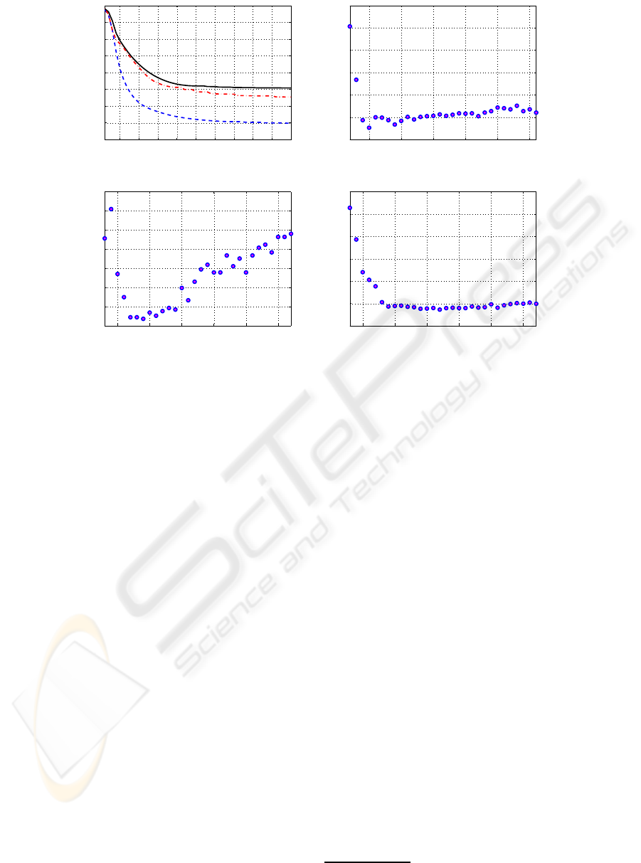
-correction rate. Figure 1(a) illustrates convergence
of Algorithm 1. Figure 2 illustrates matrices B as an
outcome of Algorithm 1.
BIOINFORMATICS 2010 - International Conference on Bioinformatics
148

5 10 15 20 25 30 35 40 45 50
0.2
0.3
0.4
0.5
0.6
0.7
0.8
0.9
1
(a): global iteration
L(A,B)
5 10 15 20 25 30
0.1
0.15
0.2
0.25
0.3
0.35
0.4
(b): number of metagenes (colon)
ALMR
5 10 15 20 25 30
0.06
0.07
0.08
0.09
0.1
0.11
0.12
0.13
(c): number of metagenes (lymphoma)
ALMR
5 10 15 20 25 30
0
0.1
0.2
0.3
0.4
0.5
0.6
(d): number of metagenes (Khan)
ALMR
Figure 1: From the top: (a) behavior of the target (2) as a function of global iteration (see global cycle in Algorithm 1), used
k = 10 - number of metagenes; dashed blue, solid black and dot-dashed red lines correspond to the colon, leukaemia and
lymphoma cases. LMRs as a function of number of metagenes, where the following schemes were used in the experiments:
(b) SCH(20,SVM,LOO); (c-d) SCH(20,MLR,LOO), see Section 4.
2.2 Multinomial Logistic Regression
(MLR)
Following (Bohning, 1992) let us consider maximi-
sation of the log-likelihood applied to the matrix B
which was produced as an outcome of Algorithm 1:
R(W) =
n
∑
j=1
"
m
∑
ℓ=1
y
jℓ
u
jℓ
− log(1+
m
∑
ℓ=1
exp(u
jℓ
)
#
,
where y
jℓ
= 0 for all ℓ = 1, ... ,m + 1, besides one i
with y
ji
= 1, W is a m×k matrix of linear coefficients,
the matrix U with elements u
jℓ
is defined as a product
WB
Our task is to find a solution for the equation
∇R(W) = 0, which represents necessary condition of
an optimum.
The following equation is called Newton’s step
and may be used as a base for the iterative algorithm
W
(s+1)
c
= W
(s)
c
− ∇
2
R(W
(s)
)
−1
∇R(W
(s)
), (5)
where ∇R is a mk- dimensional vector column (gra-
dient), and ∇
2
R is a mk- dimensional squared matrix
of second derivatives (known as Hessian matrix). All
necessary details regarding computation of the gradi-
ent vector ∇R and Hessian matrix ∇
2
R in the terms
of Kronecker products may be found in (Bohning,
1992). There is a direct correspondence between ma-
trix W and the mk-dimensional vector-column W
c
,
where first m elements of W
c
coincide with elements
of the first row of the matrix W and so on.
Note that the inverse Hessian matrix in (5) may
not exist, and, anyway, computation of an inverse ma-
trix may be a very difficult task in the case if dimen-
sion is high. We propose the following alternative up-
date procedure: W
(s+1)
c
= W
(s)
c
− v, where v is mk-
dimensional vector-column as a solution of the regu-
larised squared minimisation problem
µv
T
v+ k∇
2
R(W
(s)
)v− ∇R(W
(s)
)k
2
,
where µ is a ridge parameter for the regularisation
term. Note that regularisation term is a very impor-
tant in order to stabilise solution and reduce overfit-
ting, see for more details (Mol et al., 2009). We used
in our experiments value µ = mk/100.
3 DATA
The colon dataset
1
is represented by a matrix of 62
tissue samples (40 negative and 22 positive) and 2000
1
http://microarray.princeton.edu/oncology/affydata/
index.html
ON THE GRADIENT-BASED ALGORITHM FOR MATRIX FACTORIZATION APPLIED TO DIMENSIONALITY
REDUCTION
149

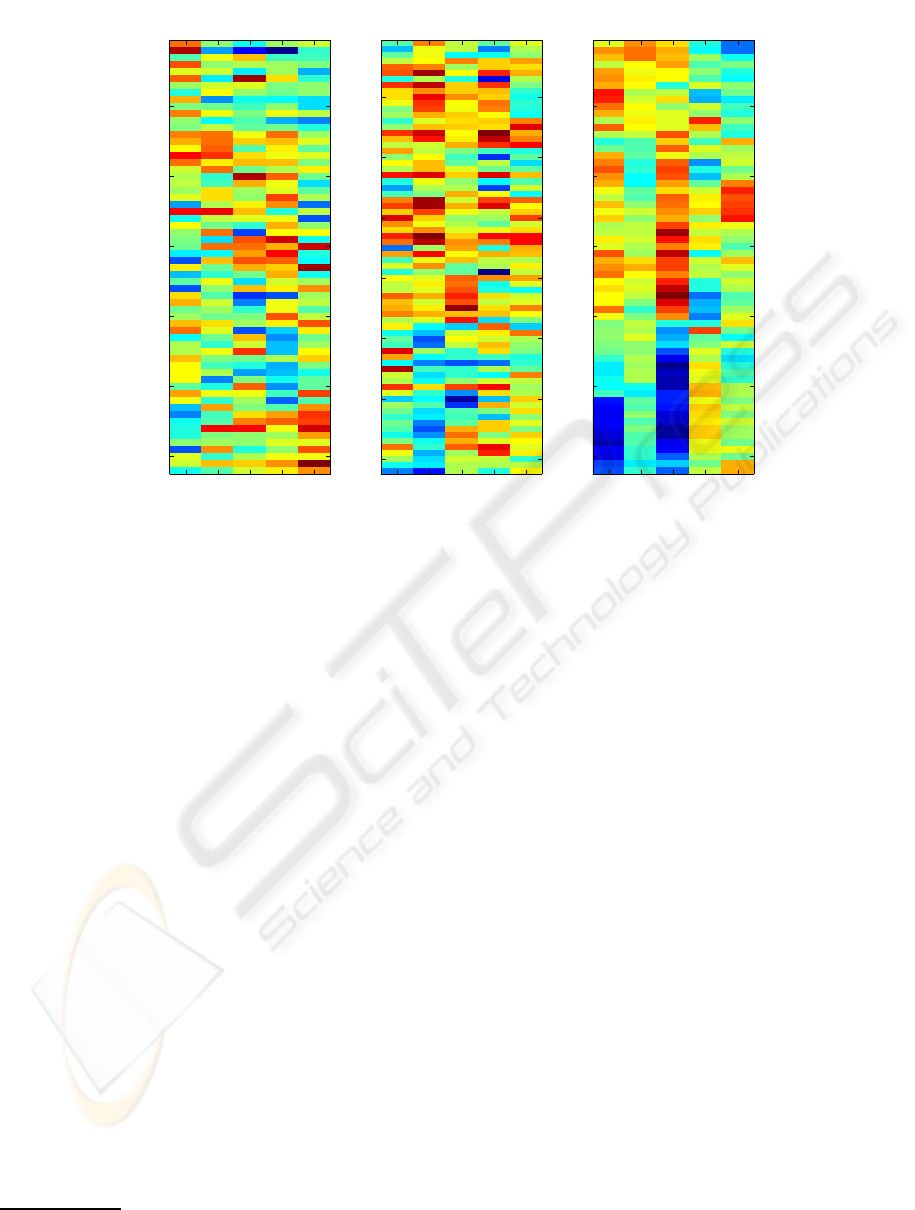
(a):metagene (colon)
tissue
1 2 3 4 5
10
20
30
40
50
60
(b):metagene (leukaemia)
tissue
1 2 3 4 5
10
20
30
40
50
60
70
(c):metagene (lymphoma)
tissue
1 2 3 4 5
10
20
30
40
50
60
Figure 2: Images of the matrix B in (1), k = 5: (a) colon (sorted from the top: 40 positive then 22 negative), (b) leukaemia
(sorted from the top: 47 ALL, then 25 AML) and (c) lymphoma (sorted from the top: 42 DLCL, then 9 FL, last 11 CLL). All
three matrices were produced using Algorithm 1 with 100 global iterations as it was described in Section 2.1.
genes. The microarray matrix for this set thus has
p = 2000 rows and n = 62 columns.
The leukaemia dataset
2
contains the expression
levels of p = 7129 genes of n = 72 patients, among
them, 47 patients suffer from acute lymphoblastic
leukaemia (ALL) and 25 patients suffer from the
acute myeloid leukaemia (AML).
We followed the pre-processing steps of (Dudoit
et al., 2002) applied to the leukaemia set: 1) thresh-
olding: floor of 1 and ceiling of 20000; 2) filtering:
exclusion of genes with max / min ≤ 2 and (max -
min) ≤ 100, where max and min refer respectively
to the maximum and minimum expression levels of
a particular gene across a tissue sample. This left us
with p = 1896 genes. In addition, the natural loga-
rithm of the expression levels was taken.
The lymphoma dataset
3
contains the gene expres-
sion levels of the three most prevalent adult lym-
phoid malignancies: (1) 42 samples of diffuse large
B-cell lymphoma (DLCL), (2) 9 samples of follicular
lymphoma (FL), and (3) 11 samples of chronic lym-
phocytic leukaemia (CLL). The total sample size is
n = 62 and p = 4026 genes. More information on
these data may be found in (Alizadeh et al., 2000).
Khan dataset (Khan et al., 2001) contains 2308
2
http://www.broad.mit.edu/cgi-bin/cancer/publications/
3
http://llmpp.nih.gov/lymphoma/data/figure1
genes and 83 observations, each from a child who
was determined by clinicians to have a type of small
round blue cell tumour. This includes the following
four classes: neuroblastoma (N), rhabdomyosarcoma
(R), Burkitt lymphoma (B) and the Ewing sarcoma
(E). The numbers in each class are: 18 - N, 25 - R, 11
- B and 29 - E.
We applied double normalisation to the data.
Firstly, we normalised each column to have means
zero and unit standard deviations. Then, we applied
the same normalisation to each row.
4 EXPERIMENTS
After decomposition of the original matrix X accord-
ing to (1), we used the leave-one-out (LOO) classifi-
cation scheme, applied to the matrix B. This means
that we set aside the ith observation and fit the clas-
sifier by considering remaining (n − 1) data points.
The experimental procedure has heuristic nature and
its performance depends essentially on the initial set-
tings (see, also, (Brunet et al., 2004)). Let us denote a
classification scheme by
SCH(nrs,Model,LOO), (6)
where we conducted nrs identical experiments with
randomly generated initial settings. Any particular
BIOINFORMATICS 2010 - International Conference on Bioinformatics
150

Table 1: Some selected experimental results, where “NM” is the number of mis-classified samples; “ls”, “SVM” and “MLR”
indicate “lscov” function in Matlab, linear SVM and multinomial logistic regression.
Data Model k AMR NM m AUC
Colon ls 5 0.1129 7 1 0.8823
Colon SVM 5 0.0968 6 1 0.8818
Leukaemia SVM 3 0.0139 1 1 0.9916
Leukaemia ls 4 0.0139 1 1 0.9957
Leukaemia SVM 35 0.0 0 1 1.0
Lymphoma MLR 12 0.0322 2 2 -
Khan MLR 21 0.0241 2 3 -
experiment includes two steps: 1) dimensionality re-
duction with Algorithm 1; 2) LOO evaluation with
classification Model. In most of our experiments with
the scheme (6) we used nrs = 20. We conducted ex-
periments with three different classifiers: 1) Matlab-
based lscov function, 2) linear SVM, and 3) we used
MLR in application to the lymphoma and Khan sets.
These classifiers are denoted by “Model” in (6).
We used two evaluation criteria: 1) LOO misclas-
sification rate (LMR) and 2) area under receiver oper-
ation curve (AUC), where the last one was used only
in application to colon and leukaemia set with binary
labels.
By definition, LMR =
1
m
∑
m
j=1
I{q
j
6= y
j
}, where
q
j
is the prediction for the label y
j
, I is an indicator
function.
Remark 2. Figures 1(b-c) illustrate average LMRs
as a function of numbers of metagenes. As it may
be expected, results corresponding to the small num-
ber of metagenes are poor because of over-smoothing.
Then, we have some improvement to some point. Af-
ter, that point the model suffers from overfitting. This
property may be used for the selection of the number
k of metagenes.
Table 1 represents some best results. It can be seen
that our results are competitivewith those in (Dettling
and Buhlmann, 2003), (Peng, 2006), where the best
reported result for the colon set is LMR = 0.113, and
LMR = 0.0139 for the leukaemia set.
The appearance of the images in Figure 2 is very
logical. We sorted the tissues in order to consider vi-
sual differences between the patterns. In the case of
the colon data, Figure 2(a), we cannot see clear sepa-
ration of the negative and positive classes. In contrast,
in the case of leukaemia, Figure 2(b), metagene N2
(from the left) separates top the 42 tissues from the
remaining 25 tissues with only one exception. It is
tissue N58 (from the top) -the only one mis-classified
tissue in Table 1 (cases k = 3, 4). Similarly, in the
case of lymphoma, Figure 2(c), metagene N1 (from
the left) separates clearly CLL from the two remain-
ing classes. Further, metagene N3 separates DLCL
from the two remaining classes.
Remark 3. In the Fig. 1(b-c) we have plotted the
average LMRs estimated using LOO cross-validation
under assumption that the matrix factorization will be
the same during the n validation trials as chosen on
the basis of the full data set. However, there will
be a selection bias in these estimates as the matrix
factorization should be reformed as a natural part of
any validation trial; see, for example, (Ambroise and
McLachlan, 2002). But, since the labels y
t
of the
training data were not used in the factoring process,
the selection bias should not be of a practical impor-
tance.
4.1 Computation Time
A Linux computer with speed 3.2GHz, RAM 16GB,
was used for most of the computations. The time for
300 global iterations with Algorithm 1 (used special
code written in C) in the case of k = 11 was between
10 and 15 sec. Based on our experiments, 20 global
iterations with non-negative matrix factorization (Lee
and Seung, 2000) for the same task as above requires
about 25 min.
5 CONCLUSIONS
Microarray data analysis is challenging the traditional
machine learning techniques due to the availability of
a limited number of training instances and the exis-
tence of large number of genes, together with the in-
herent various uncertainties. In many cases machine
learning techniques rely too much on the gene selec-
tion, which may cause selection bias. Generally, fea-
ture selection may be classified into two categories
based on whether the criterion depends on the learn-
ing algorithm used to construct the prediction rule. If
the criterion is independent of the prediction rule, the
ON THE GRADIENT-BASED ALGORITHM FOR MATRIX FACTORIZATION APPLIED TO DIMENSIONALITY
REDUCTION
151

method is said to follow a filter approach, and if the
criterion depends on the rule, the method is said to
follow a wrapper approach (Ambroise and McLach-
lan, 2002). The objective of this study is to develop
a filtering machine learning approach and produce a
robust classification for microarray data.
Based on our experiments, the proposed matrix
factorisation performed an effective dimensional re-
duction as a preparation step for the following su-
pervised classification. Classifiers built in metagene,
rather than original gene, space are more robust and
reproducible because the projection can reduce noise
more than simple normalisation. Algorithm 1, as a
main contribution of this paper, is conceptually sim-
ple. Consequently, it is much faster compared to pop-
ular NMF. Stability of the algorithm depends essen-
tially on the properly selected learning rate, which
must not be too big. We can include additional func-
tions so that the learning rate will be reduced or in-
creased depending on the current performance.
There are many advantages to such a metagene
approach. By capturing the major, invariant biolog-
ical features and reducing noise, metagenes provide
descriptions of data sets that allow them to be more
easily combined and compared. In addition, interpre-
tation of the metagenes, which characterize a subtype
or subset of samples, can give us insight into underly-
ing mechanisms and processes of a disease.
The results that we obtained on three real datasets
confirm the potential of our approach.
REFERENCES
Alizadeh, A., Eisen, M., Davis, R., Ma, C., Lossos, I.,
Rosenwald, A., Boldrick, J., Sabet, H., Tran, T., and
Yu, X. (2000). Distinct types of diffuse large b-
cell-lymphoma identified by gene expression profil-
ing. Nature, 403:503–511.
Ambroise, C. and McLachlan, G. (2002). Selection bias in
gene extraction on the basis of microarray gene ex-
pression data. Proceedings of the National Academy
of Sciences USA, 99:6562–6566.
Bohning, D. (1992). Multinomial logistic regression algo-
rithm. Ann. Inst. Statist. Math., 44(1):197–200.
Brunet, J., Tamayo, P., Golub, T., and Mesirov, J. (2004).
Metagenes and molecular pattern discovery using
matrix factorisation. Proceedings of the National
Academy of Sciences USA, 101(12):4164–4169.
Dettling, M. and Buhlmann, P. (2003). Boosting for tumor
classification with gene expression data. Bioinformat-
ics, 19(9):1061–1069.
Dudoit, S., Fridlyand, J., and Speed, I. (2002). Comparison
of discrimination methods for the classification of tu-
mors using gene expression data. Journal of Americal
Statistical Association, 97(457):77–87.
Guyon, I., Weston, J., Barnhill, S., and Vapnik, V. (2002).
Gene selection for cancer classification using support
vector machines. Machine Learning, 46:389–422.
Khan, J., Wei, J., Ringner, M., Saal, L., Ladanyi, M., West-
ermann, F., Berthold, F., and Schwab, M. (2001).
Classification and diagnostic prediction of cancers us-
ing gene expression profiling and artificial neural net-
works. Nature Medicine, 7(6):673–679.
Koren, Y. (2009). Collaborative filtering with temporal dy-
namics. In KDD, pages 447–455.
Lee, D. and Seung, H. (2000). Algorithms for non-negative
matrix factorisation. In Advances in Neural Informa-
tion Processing Systems.
Mol, C., Mosci, S., Traskine, M., and Verri, A. (2009). A
regularised method for selecting nested groups of rel-
evant genes from microarray data. Journal of Compu-
tational Biology, 16(5):677–690.
Peng, H. and Ding, C. (2005). Minimum redundancy and
maximum relevance feature selection and recent ad-
vances in cancer classification. In SIAM workshop on
feature selection for data mining, pages 52–59.
Peng, Y. (2006). A novel ensemble machine learning for
robust microarray data classification. Computers in
Biology and Medicine, 36:553–573.
Tamayo, P., Scanfeld, D., Ebert, B., Gillette, M., Roberts,
C., and Mesirov, J. (2007). Metagene projection
for cross-platform, cross-species characterization of
global transcriptional states. Proceedings of the Na-
tional Academy of Sciences USA, 104(14):5959–5964.
Zhang, X., Lu, X., Shi, Q., Xu, X., Leung, H., Harris, L.,
Iglehart, J., Miron, A., and Wong, W. (2006). Re-
cursive svm feature selection and sample classifica-
tion for mass-spectrometry and microarray data. BMC
Bioinformatics, 7(197).
BIOINFORMATICS 2010 - International Conference on Bioinformatics
152