
INTELLIGENT VISION FOR MOBILE AGENTS
Contour Maps in Real Time
Tariq Khan, John Morris and Khurram Jawed
Electrical and Computer Engineering, The University of Auckland, Auckland, New Zealand
Keywords:
Contour maps, Real time stereo, Dynamic scene navigation.
Abstract:
Real time interpretation of scenes is a critical capability for fast-moving intelligent vehicles. Generation of
contour maps from stereo disparity maps is one technique which allows rapid identification of objects. Here,
we describe an algorithm for generating contour maps from disparity maps produced using an implementation
of the Symmetric Dynamic Programming Stereo algorithm in an FPGA. The algorithm has three steps: (a)
a median filter is applied to the disparity map to remove the streaks characteristic of dynamic programming
algorithms, (b) irrelevant pixels in the centre of regions are marked and (c) selected contours outlined. Results
for high resolution images (∼ 1Mpixel) show that a number of critical contours can be generated in less than
30ms permitting object outlining at video frame rates. The algorithm is easily parallelized and we show that
multiple core processors can be used to increase the number of contours that can be generated.
1 PREAMBLE
Current state-of-the-art processors do not have suf-
ficient processing power to process high resolution
stereo pairs with large disparity ranges in real time.
To solve this problem, we implemented the Symmet-
ric Dynamic Programming Stereo (SPDS) algorithm
(Gimel’farb, 2002) in reconfigurable hardware: our
system generates disparity and occlusion maps from
one megapixel images in real-time (30fps) (Jawed
et al., 2009; Morris and Gimel’farb, 2009). This
leaves the host processor free to interpret the dispar-
ity maps and add the ability to recognize and track
objects in complex dynamic scenes in real time. As
a first step to adding real intelligence to a mobile
agent (intelligent mobile robot, autonomous automo-
bile, etc.), we describe a contour map generation al-
gorithm which processes the disparity maps produced
by the SDPS hardware in real time. Whereas tradi-
tional segmentation approaches will generate multi-
ple segments for a textured object which then need
to be merged using other information (e.g. optical
flow), generation of the contour maps (effectively a
segmentation of the disparity map) directly generates
information about the object geometry which can be
used for recognition or tracking.
1.1 Related Work
Active contour techniques which try to fit contours to
image features are well known but they have several
drawbacks: they are sensitive to initialization, may
stop on incorrect local minima and do not handle tex-
tured backgrounds containing multiple objects at all
(Kass et al., 1988; Williams and Shah, 1992; Xu and
Prince, 1998). Kim et al. used a similar approach on
disparities derived from stereo pairs but they were un-
able to obtain real time performance (Kim et al., 2005;
Kim et al., 2006).
2 SYMMETRIC DYNAMIC
PROGRAMMING STEREO
We include here a brief description of the SDPS algo-
rithm, highlighting its characteristics which are rel-
evant to the current work. A key difference in its
approach is that, rather than create a disparity map
corresponding to the left or right image as the refer-
ence image, it creates the disparity map that would be
seen by a Cyclopæan ‘eye’ placed midway between
the two cameras. This enables it to place some vis-
ibility constraints on the allowed transitions between
states for each pixel. Examination of Figure 1 shows
391
Khan T., Morris J. and Jawed K. (2010).
INTELLIGENT VISION FOR MOBILE AGENTS - Contour Maps in Real Time.
In Proceedings of the 2nd International Conference on Agents and Artificial Intelligence - Artificial Intelligence, pages 391-397
DOI: 10.5220/0002738503910397
Copyright
c
SciTePress
p=3
B B
B
B ML
p=6
p=5
p=4
O
L
O
R
O
C
4 5 63210 4 5 63210
3 5 974 6 8
MR
ML
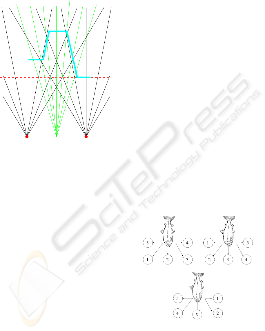
Figure 1: SDPS ‘view’ showing part of the Cyclopæan im-
age seen by the virtual Cyclopæan camera (centre) and a
scene object profile. Visibility states (ML, B or MR) are
marked on the profile. Even if there is an abrupt change in
disparity, SDPS, in common with other stereo correspon-
dence algorithms, cannot distinguish between the triangular
profile shown here and the one with an abrupt change.
that, in the Cyclopæan image, a transition between
two disparity levels, p
1
and p
2
, should result in ex-
actly |p
1
− p
2
| occluded pixels marked ML (monoc-
ular left) or MR (monocular right) in the diagram in
the Cyclopæan image. This simplifies for the hard-
ware implementation: the predecessor array elements
are only two bits each - encoding the ML, MR or B
(binocularly visible) state on each path - and saving
space for the most ‘expensive’ element of the whole
circuit. The dynamic programming back-track, which
generates the optimal path, relies on the state tran-
sition rules(Gimel’farb, 1991) to generate the stream
of disparities. The hardware implementation is fully
described elsewhere(Morris et al., 2009; Morris and
Gimel’farb, 2009; Jawed et al., 2009). An additional
feature of the SDPS algorithm is that it generates oc-
clusion maps at no additional cost: they are a natural
by-product of the SDPS algorithm(Morris et al., 2009;
Gimel’farb, 1991). They clearly outline objects in the
scene and, as we show here, useful to speed up scene
interpretation.
3 CONTOUR MAP GENERATION
We process the disparity maps generated by the SDPS
hardware in three steps: two pre-processing steps -
median filtering (see Section 3.1) and C-state assign-
ment (see Section 3.2) - followed by the ‘Salmon’
algorithm which generates the contour maps them-
selves, described in Section 4.
3.1 Median Filtering
SDPS, like other dynamic programming stereo algo-
rithms, produces ‘streaks’ in the disparity maps be-
cause the occlusion penalty prevents a change in dis-
parity. Since these streaks often occupy a single scan
line, most of them are removed by applying a vertical
median filter to the generated disparity map.
3.2 C-state Assignment
In this phase, pixels are classified according to their
visibility states:
B binocularly visible - seen by both cameras
ML monocular left - seen by the left camera only
MR monocular right - seen by the right camera
only
C centre - of regions of equal disparity
The first three are the same states that the SDPS
algorithm uses. The ‘C’ state is added to classify
pixels which cannot lie on contour lines and are
ignored in most steps of the Salmon algorithm.
ON-EDGE INSIDE
OUTSIDE
Figure 2: Order in which the neighbours are visited for each
of the three salmon states for a salmon ‘descending’ (π ≤
θ ≤ 2π) an ML edge. The order is reversed for a salmon
‘climbing’ (0 ≤ θ ≤ π) an MR edge.
ICAART 2010 - 2nd International Conference on Agents and Artificial Intelligence
392

4 SALMON
Our algorithm is modeled on the incredible journey
of a salmon downstream to the ocean, returning the
same spot as an adult
1
: our salmon leaves a trail of
points behind it as it traces the contour and returns to
its starting place.
For any given contour at disparity p, choose the first
ML point from the first scan line with a point at dis-
parity p in the linked list generated when C states
were assigned.
Denote the salmon’s current location by P
c
and the
disparity at P
c
by p
c
. The salmon states during con-
tour generation are designated ON − EDGE, INSIDE
or OUTSIDE. Table 1 defines these states.
The salmon’s full state is defined by a 4-tuple:
(s, p
s
, up, r
max
)
where s ∈ {ON − EDGE, INSIDE, OUTSIDE} is
the salmon state, p
s
is the disparity for which the
salmon is constructing a contour, up is either true
(tracing MR contour) or false (tracing ML contour)
and r
max
is maximum extent of the salmon’s sight -
a measure of how many neighbours the salmon will
examine in this iteration. For sight, j| j = 1, ..., r
max
,
the salmon will examine N = 4 j + 1 neighbours. The
directions of the neighbours, φ
i
are defined by:
φ
0
= when (up = true) 0 else π
φ
i
= φ
i−1
+
π
4 j
, i = 1, 2, . . . , N
where φ = 0 represents the direction along the x axis
and φ increases in an anti-clockwise direction.
The salmon’s initial state will be ON-EDGE. Our
salmon then follows the p
s
contour and returns to
where it started: it uses rules derived from the vis-
ibility constraints (Gimel’farb, 1991). From an MR
pixel, the salmon moves up - 0 ≤ φ ≤ π. From an ML
pixel, the salmon moves down so that π ≤ φ ≤ 2π. The
salmon uses steps j = 1, .., r
max
to decide in which di-
rection it should move. If it can not decide at step j
then it tries step j + 1.
4.1 General Rules
1. Any point in C state is ignored.
2. A neighbour at j always has higher priority than
neighbours at j + 1.
1
”Salmon make an incredible journey downstream
from the fresh water where they are born, to the
ocean, and then back upstream again as adults,
finding the exact location where they began sev-
eral years earlier.” (U.S. Bureau of Land Manage-
ment http://www.blm.gov/education/00_resources/
articles/Columbia_river_basin/posterback.html)
3. Transition to an ON-EDGE state always has high-
est priority.
4. Transition to an INSIDE state always takes prior-
ity over transition to an OUTSIDE state.
5. If there are two or more possible transitions to IN-
SIDE neighbours than the neighbour with closest
disparity will be chosen.
6. If there are two or more possible transitions to
OUTSIDE neighbours than the neighbour with
closest disparity will be chosen.
7. If the current state is ON-EDGE or INSIDE then
ML or MR is chosen over B with same disparity.
8. If the current state is OUTSIDE then B is chosen
over ML or MR with the same disparity.
4.2 Search Priority
For each salmon state, the order in which the neigh-
bours are searched is different: the priorities for the
salmon moving down and for j = 1 are shown in Fig-
ure 2.
4.3 Expanding the Search Region
If all the neighbours of a point are marked C or have
been visited, then we increment j and search in a
wider region. To prevent the salmon from selecting
the wrong neighbour, a maximum iteration count is
specified. If this count reaches a predefined limit or
the salmon returns to its starting point, the contour
will be terminated and added to the contour list.
4.4 Salmon Operation
An example salmon run is shown in Figure 3. The
salmon starts in the (7,ML) pixel at the top and works
down, trying to stay on the (7,ML) ‘edge’.
However, it is not possible always: in row 2, the
salmon is ON-EDGE, but there is no (7,ML) neigh-
bour, so the salmon will use the priority scheme
shown in Figure 2 and go INSIDE to (8,B) attempting
to find another (7, ML) point.
In row 4 at (7, ML), again there is no adjacent (7, ML)
so the salmon will go OUTSIDE to (6, B) and follow
the priorities shown in Figure 2 to find (7,ML) again.
Then a sequence of (7,ML) pixels are followed until
at row 9, the salmon is facing a continuous wall of C
pixels. It is forced to go INSIDE and swim through
a sequence of (7,B) pixels (a horizontal edge), even-
tually finding a (7, MR) one. At this point, it reverses
the direction and ‘climbs’ the (7, MR) edge back to
the starting point.
INTELLIGENT VISION FOR MOBILE AGENTS - Contour Maps in Real Time
393
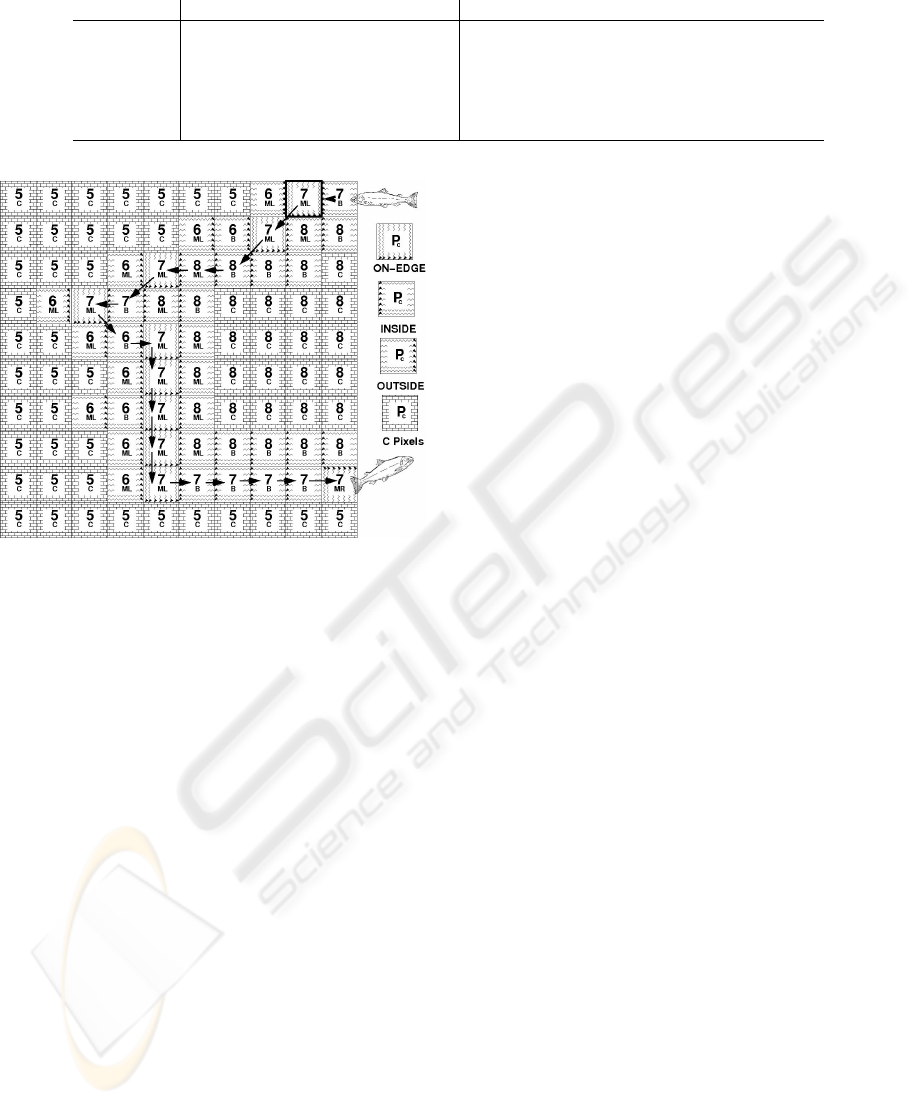
Table 1: Salmon state definitions.
State Definition Action
ON-EDGE on an edge: P
c
is in ML or MR state
with p
c
= p
s
continue along the edge
INSIDE inside a contour: P
c
is in B state
with disparity equal to p
s
or p
c
> p
s
when going (down | up), go outwards (to the
(le f t | right)) to find the p
s
edge
OUTSIDE outside: p
c
< p
s
when going (down | up), go inwards (to the
(right | le f t)) to find the p
s
edge
Figure 3: Example Salmon ‘run’: boxes represent pixels
in the disparity and occlusion maps - they are labeled with
the disparity and the visibility state after C states have been
assigned. The background pattern for each pixel shows
the salmon state as it visits a pixel - see the legend. The
salmon starts with the highlighted (7,ML) pixel at the top,
‘descends’ through ML pixels and climbs back (not shown)
through MR pixels to reach its starting point again.
4.5 Horizontal Edges
Objects with horizontal edges present the largest chal-
lenge to the Salmon algorithm: they show large dis-
parity jumps between scanlines and can have large
regions of B pixels adjacent to B pixels with a dif-
ferent disparity, i.e. there are no ML or MR pixels
delineating the contour. A disparity map for a syn-
thetic scene with horizontal edges is shown in Figure
4. Figure 5(a)-(h) shows in detail the behaviour at
each transition to a horizontal edge. Note that when
there are large disparity changes in the vertical direc-
tion, several contours will, as expected, run through
the same pixels. In Figure 5(a), the p = 6 contour en-
ters the INSIDE state and then turns left, preferring
the (6,B) pixels over the (6,C) pixels (which must con-
stitute the centre of a plane). This contour will even-
tually encounter (6,ML) pixels (Figure 5(e)) enter the
ON-EDGE state and continue normally. The p = 7
contour prefers the (8,ML) pixel to its right (rule 4
because the (6,B) pixel would be an OUTSIDE state
for it) and follows the (8,B) pixels in an INSIDE state
until it encounters a (7,MR) pixel (Figure 5(b)) and
changes direction. The p = 8 contour also prefers the
(8,B) pixel because the (7,ML) pixel is OUTSIDE for
it.
In Figure 5(b), the p = 8 and p = 7 contours find
their correct MR ‘edges’, separate and climb the MR
edge. The p = 6 contour reaches a (6,MR) pixel and
climbs. In Figure 5(c), three contours find walls of
C pixels and choose to follow the (8,B) pixels (rule
1). In Figure 5(d), three contours locate their starting
points (outlined in black) and terminate. Figure 5(d) -
(h) show a single contour avoiding a wall of C pixels.
5 RESULTS
In Table 2, we show times for pre-processing a 1024 ×
768 pixel image, whose disparity map produced by
the SDPS hardware has 2048 × 768 pixels (a conse-
quence of the Cyclopæan view). These stages are
readily parallelized and the times for a quad core pro-
cessor are well within our target of 30 ms for real
time performance at 30fps. The contour generation
code was compiled using Visual C++’s optimizers but
little attempt was made to optimize the C code it-
self. Median filtering and C state assignment could
also be sped up by using the MMX hardware within
each processor, so further improvements are certainly
possible. Since generating a set of 24 contours for
an ∼ 1Mpixel image is taking less than 10 ms, there
is significant scope for object recognition or tracking
capabilities to be added whilst maintaining real time
performance.
Selected frames from two image sequences are shown
in Figure 6 and Figure 7. In the first set, two con-
tours are shown - the ball and the thrower. Note
that the contour has correctly identified the thrower
as leaning forward slightly - not chopped his legs off!
In the second set, we demonstrate the capability of
our hardware-software combination to capture a small
fast moving silicone rubber ball in flight!
ICAART 2010 - 2nd International Conference on Agents and Artificial Intelligence
394

Figure 4: Disparity map for scene object with horizontal edges: the marked regions are shown in detail in Figure 5.
(a) (b) (c)
(d) (e) (f)
(g) (h)
Figure 5: Salmon operation for the regions marked in Figure 4.
6 CONCLUSIONS
Using high resolution disparity maps (original im-
ages: 1024 × 768 pixels with disparity range of 80)
produced in real time (30 fps) by an FPGA based
attached processor, the salmon is able to generate a
INTELLIGENT VISION FOR MOBILE AGENTS - Contour Maps in Real Time
395
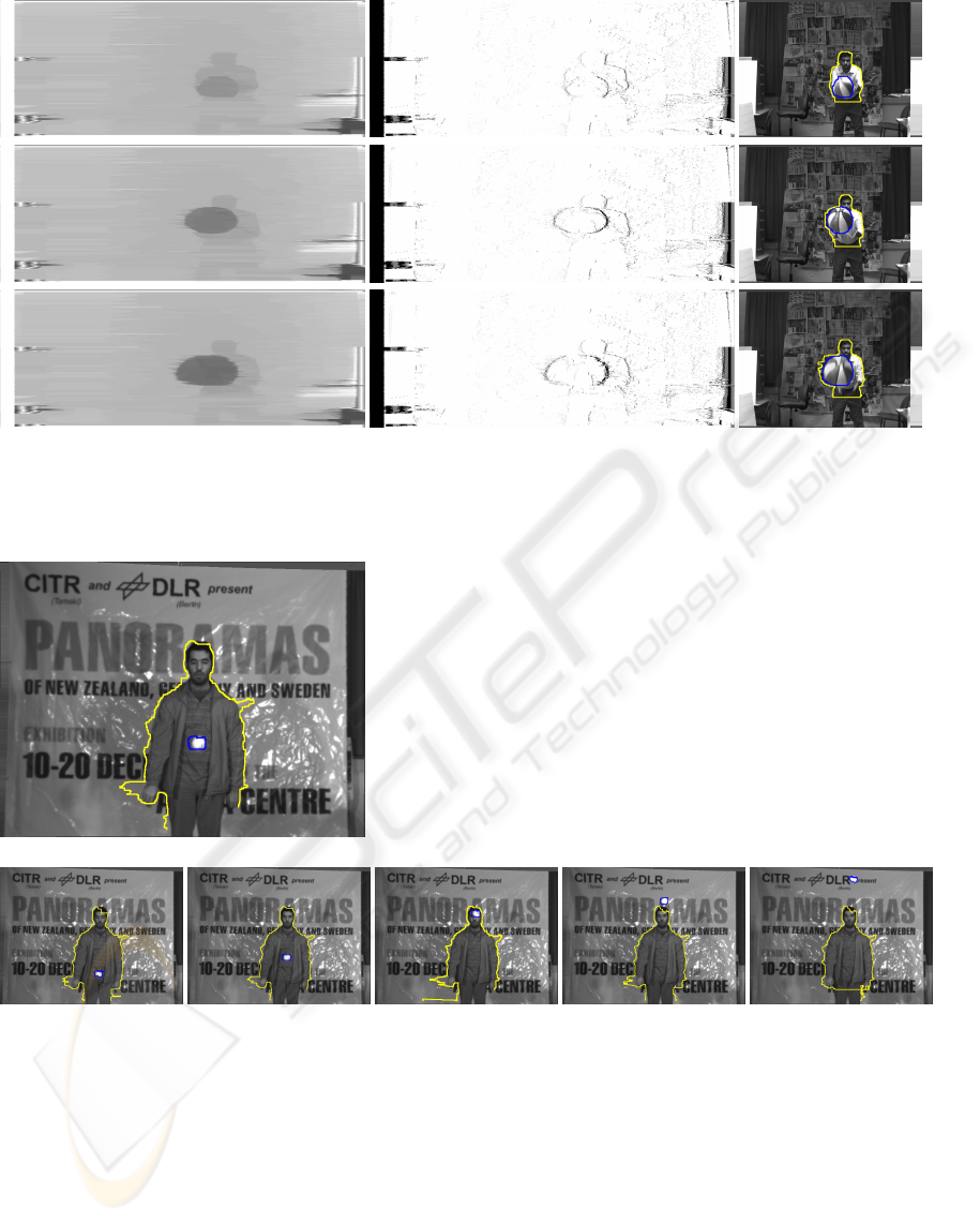
Disparity map Occlusion map Contour map (L image)
Figure 6: Example contours - Basket ball sequence: frame rate - 30fps: two sample contours are shown for each frame. Note
that the maps are twice as wide as the original image: the SDPS algorithm produces a Cyclopæan view with twice as many
points as the original images.
Original scene
Figure 7: Example contours - silicone ball sequence. A small silicone ‘bouncy’ ball is captured in flight in the lower slices
taken from the full scene (top image). The thrower and the ball are outlined. Colour images of both these and other sequences
can be viewed at http://www.cs.auckland.ac.nz/
˜
jmor159/HRPG/RT/index.html.
number of critical contour maps in real time. The time
to generate each contour is proportional to its length
but the algorithm generates each contour indepen-
dently and is able to use the multiple cores commonly
available now to advantage. Most of the processing
time is used in median filtering and C state assign-
ment: these tasks are regular and good candidates for
implementation on the FPGA - freeing further CPU
cycles for generating additional contours, matching
contours to object profiles or tracking objects outlined
by contours. The current SDPS implementation is
very efficient and uses only a fraction of the resources
available in modern FPGAs(Jawed et al., 2009) so
that additional processing on the FPGA surface is pos-
sible. Additional FPGA processing will add a small
latency to the time between image capture at the cam-
ICAART 2010 - 2nd International Conference on Agents and Artificial Intelligence
396

Table 2: Execution time.
Median filtering
Window Number of Cores
size 1 2 3 4
1 × 3 25 15 11 9
1 × 5 31 17 13 9
1 × 7 35 20 14 11
1 × 9 39 22 15 12
1 × 11 42 23 16 13
1 × 13 45 25 17 14
1 × 15 48 27 18 16
1 × 17 51 28 20 15
1 × 19 52 30 20 16
C state assignment 6 5 4 3.7
Contour Generation
Disparity Number
set of points
13-36 37208 8.4 7.2 6.3 -
All times in milliseconds for a 2.4GHz quad core
processor.
era and receipt of scan lines in the host processor: at
most the number of scan lines in the median filter win-
dow - typically less than 1 ms of real time.
REFERENCES
Gimel’farb, G. (1991). Intensity-based computer binocu-
lar stereo vision: signal models and algorithms. Int J
Imaging Systems and Technology, 3:189–200.
Gimel’farb, G. (2002). Probabilistic regularisation and
symmetry in binocular dynamic programming stereo.
Pattern Recognition Letters, 23(4):431–442.
Jawed, K., Morris, J., Khan, T., and Gimel’farb, G. (2009).
Real time rectification for stereo correspondence. In
Xue, J. and Ma, J., editors, 7th IEEE/IFIP Intl Conf
on Embedded and Ubiquitous Computing (EUC-09),
pages 277–284. IEEE CS Press.
Kass, M., Witkin, A., and Terzopoulos, D. (1988). Snakes:
Active contour models. International Journal of Com-
puter Vision, 1(4):321–331.
Kim, S. H., Alattar, A., and Jang, J. W. (2006). Object con-
tour tracking using the optimization of the number of
snake points. In Int Conf on Computational Intelli-
gence and Security, volume 2.
Kim, S. H., Jang, J. W., Lee, S. P., and Choi, J. H.
(2005). Accurate contouring technique for object
boundary extraction in stereoscopic imageries. LNCS,
3802:869.
Morris, J. and Gimel’farb, G. (May 6, 2009). Real-time
stereo image matching system. NZ Patent Application
567986.
Morris, J., Jawed, K., and Gimel’farb, G. (2009). Intel-
ligent vision: A first step - real time stereovision.
In Advanced Concepts for Intelligent Vision Systems
(ACIVS’2009), volume 5807 of LNCS, pages 355–
366. Springer.
Williams, D. J. and Shah, M. (1992). A fast algorithm for
active contours and curvature estimation. CVGIP: Im-
age understanding, 55(1):14–26.
Xu, C. and Prince, J. L. (1998). Snakes, shapes, and gradi-
ent vector flow. Image Processing, IEEE Transactions
on, 7(3):359–369.
INTELLIGENT VISION FOR MOBILE AGENTS - Contour Maps in Real Time
397
