
SYNTHESIS OF DRIVING SIGNALS FOR MEDICAL IMAGING
ANNULAR ARRAYS FROM ULTRASONIC X-WAVE SOLUTIONS
L. Castellanos
1
, A. Ramos and H. Calás
Dpto. Señales, Sistemas y Tecnologías Ultrasónicas, Instituto de Acústica - CSIC, Serrano 144, 28006 Madrid, Spain
Keywords: Beam Collimation, Driving signals, X wave, Pressure field, Velocity potential.
Abstract: An interesting approach for achieving high-resolution in ultrasonic imaging, is producing in real time
limited diffraction waves with annular arrays; this potential option was presented by J.-Y. Lu in 1991 for
collimating ultrasonic beams in medical imaging, approximating classical X waves with a finite aperture 10-
annuli array, driven with 0-order X-wave excitation signal generated by solving the isotropic/homogeneous
scalar wave equation. However, detailed solutions for a proper array electrical driving in order to form X-
wave fields of both pressure and velocity potential have been not still reported. Paper objective is to show a
tool to obtain approximated solutions for the inverse problems (aspect by-passed in classical approach) of
synthesizing voltage excitations sets for producing both possible X wave field profiles, and comparatively
investigate their distinct beam collimating capacities. All calculations, simulations and analyses were made
for an ad-hoc developed 8-rings 2.5 MHz array transducer. Results show field distributions in ultrasonic
pressure, created for two driving approaches derived by our inverse processing from calculated pressure and
velocity potential fields. The good performances resulting in both cases for beam collimation, confirm the
tool applicability. Results suggest the viability of our procedure as a promising alternative to classical X-
wave driving calculations.
1 INTRODUCTION
To achieve with ultrasonic beams a high lateral
resolution for medical imaging applications, requires
conventional scanners with very complex electronic
& processing technologies for performing a multiple
focusing, of the classical phase-array type, or well to
alternatively essay new ways for beam collimation,
so searching a lower technological complexity. For
this aim, some solutions based in non-diffracting set-
ups have been proposed. One of the potentially best
options seems to be the X waves, which are derived
from theoretical limited-diffraction solutions for the
scalar wave equation in isotropic/homogeneous
media as is assumed in medical imaging. A classic
practical approach for high-resolution was presented
by J.-Y. Lu & J. F. Greenleaf in 1991 (Lu, 1991),
which take the 0-order X waves as excitation signals
for the multiple driving of an annular array. Other
alternative kind of X waves were theoretically
obtained by Shusilov et. al. (Shusilov, 2001), and Y.
Crespo et. al. (Crespo, 2005), employing the method
developed by Donelly et. al. (Donelly, 1992).
However, detailed solutions for a proper array
electrical driving, by inverse processing, in order to
form X-wave fields of both pressure and velocity
potential, have been not still reported. The main
paper objective is to overcome some aspects not
addressed in classic X-wave approach: firstly to
show in detail a reasonably approximated solution
for the inverse problems of synthesizing voltage
excitations sets, in order to produce X wave fields,
and secondly to extent it for obtaining the 0-0rder X-
wave in terms of pressure field pattern; in addition,
the respective collimating properties of both field
options are comparatively investigated.
2 THEORY
A. Potential Flow Theory
Potential flow theory describes the cinematic
behaviour of the fluids. For this theory, it is assumed
that the velocity field of flow is equal to the negative
gradient of a potential function, this potential
290
Castellanos L., Ramos A. and Calás H. (2010).
SYNTHESIS OF DRIVING SIGNALS FOR MEDICAL IMAGING ANNULAR ARRAYS FROM ULTRASONIC X-WAVE SOLUTIONS.
In Proceedings of the Third International Conference on Bio-inspired Systems and Signal Processing, pages 290-295
DOI: 10.5220/0002746802900295
Copyright
c
SciTePress

function cause the movement of the fluid, this is
write like (Strutt, 1896):
u
φ
→
=−∇ (1)
Where:
u
→
is the velocity of vector for each
medium particle,
φ
is the velocity potential field. In
accordance with the potential flow theory, the
pressure is describing like:
0
p
t
φ
ρ
∂
=
∂
(2)
Where: p is the field of pressure,
0
ρ
is the
density of medium. Then the velocity potential is:
0
1
p
t
φ
ρ
=∂
∫
(3)
B. Piezoelectric Transducer Model
A piezoelectric transducer is an especial kind of the
electro-mechanic transducers. This transducer
converting the electrical to mechanical energy and
vice-versa, is employed like a sensor as an actuator.
The complexity of the electro-mechanic process
is explicated with detail in some works (Masson,
1964), (Püttmer, 1997), (Arnau, 2004). The
simplifications assumed for these analyses are based
in the supposition of transducer working in only one
vibration mode, and the planar dimensions of the
piezoelectric material being larger than thickness. In
this work, we employ an electric model of the
Thickness Expander mode (TE) of the transducer.
This model is based in SPICE piezoelectric model,
developed by Püttmer et. al. (Püttmer, 1997).
C. Synthesizing approximated Voltage
Excitations
To approach solutions to the inverse problems of
synthesizing two voltage excitations sets, needs of
describing the conversion of driving voltage V
across input terminals to velocity u
L
in the emitting
face of transducer. For this, we take the following
equation of transducer in broadband (Arnau, 2004):
I
Cj
u
j
h
u
j
h
V
S
BL
0
3333
1
ωωω
++= (4)
If we write the equation 4 in the time domain:
∫∫∫
∂+∂+∂= tI
C
tuhtuhV
S
BL
0
3333
1
(5)
Then, V could be approximated, in broadband
operation, and under certain conditions in backing
impedance u
B
, as proportional to the integration of
the velocity in the emitting face of transducer:
∫
∂∝ tuhV
L33
(6)
D. Spatial Impulse Response Method
Spatial impulse response method (Stepanishen,
1971) has been largely applied to obtain the pressure
field under a diffraction process. For array cases, the
pressure response can be written as (Ullate, 1994):
),(*
)(
),(
1
txh
t
u
txp
k
N
k
Lk
∑
=
∂
∂
=
ρ
(7)
where p is the acoustic pressure, x is the vector
of position,
ρ
is the density of medium, u
Lk
is the
velocity in the face of the annulus k, h
k
is the spatial
impulse response of the annulus k and * represent
the time convolution operator.
E. Broadband 0-order X Wave
Equation
Because the 0-order X wave allows a more punctual
and effective collimation than other options among
the X wave family, we use, as in (Lu, 1991), this
sub-class. The expression for the 0-order X wave
family produced by an infinite aperture and
broadband conditions is (Lu, 1991):
() ( )
[]
2
0
2
0
cossin
0
ctziar
a
X
−−+
=Ψ
ζζ
(8)
where
0
X
Ψ
represents the theoretical 0-order X
wave, a
0
> 0 is a constant, r is the radial coordinate,
ζ (0< ζ <π/2) is the Axicon angle, z is the axial
distance, c is the speed of sound in the medium, and
t is the time. For our case, these parameter values
were used: a
0
= 0.05 mm, ζ = 4° and c = 1.5 mm/μs.
2 DRIVING AND FIELD RESULTS
In this work, we consider two cases for the 0-order
X waves: in pressure and in velocity potential.
The potential flow theory (Strutt, 1896) for field
aspects, and expression (6) for inverse processing,
SYNTHESIS OF DRIVING SIGNALS FOR MEDICAL IMAGING ANNULAR ARRAYS FROM ULTRASONIC
X-WAVE SOLUTIONS
291
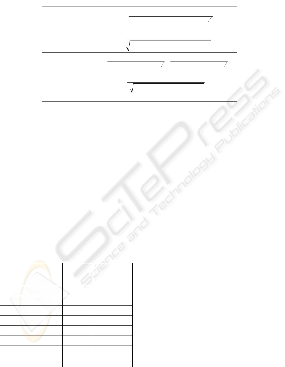
Table 1: Resume of field expressions from 0-order X-wave solution in terms of velocity potential.
0-order X wave in velocity potential.
Theoretical pressure
fields.
(
)
() ( )
{}
000
3
2
2
2
0
cos
sin cos
aic a i z ct
raizct
ρζ
ζζ
−−⎡⎤
⎣⎦
−
+− −⎡⎤
⎣⎦
Theoretical potential
velocity fields.
() ( )
0
2
2
0
sin cos
a
raizct
ζζ
+− −
⎡
⎤
⎣
⎦
Theoretical velocity
fields.
() ( )
{}
(
)
() ( )
{}
2
00
0
33
22
22
22
00
cos cos
sin
sincos sincos
ai a i z ct
ar
rz
raizct raizct
ζζ
ζ
ζζ ζζ
−−
⎡⎤
⎣⎦
−
+− − +− −⎡⎤ ⎡⎤
⎣⎦ ⎣⎦
Signals ∝ to
excitation voltages,
derived by inverse
processing .
() ( )
33 0
2
2
0
cos
sin cos
ha
K
cr a iz ct
ζ
ζζ
−
+
+− −
⎡⎤
⎣⎦
were employed to obtain the results shown in the
table 1, which includes theoretical field expressions
from X-wave solution in terms of velocity potential
and an approximate driving voltage.
When a plane array transducer is modelled as
vibrating in a thickness extensional (TE) mode, only
is possible to calculate its perpendicular velocities
field in the z direction. Thus, we only take into
account velocities in z direction in order to obtain
the proportional signals for the excitation voltages.
As it is shown in table 1, our voltage excitations, to
obtain 0-order X waves in velocity potential, are
waveforms with morphology similar to excitation
signals employed by J-Y Lu and J. F. Greenleaf in
your X-wave experimental verification (Lu, 1991).
To note that these approximated excitation signals
are also very similar to the velocity potential.
Table 2: Geometrical characteristics of each transducer
ring in the annular array transducer.
Number of
element.
Intern
Radio
[mm].
Extern
Radio
[mm].
Evaluation
value [mm].
1 0 2 0
2 2.2 4.59 3.395
3 4.79 7.2 5.995
4 7.4 9.81 8.605
5 10.01 12.4 11.205
6 12.6 15 13.8
7 15.2 17.6 16.4
8 17.8 20.3 19.05
In the figure 1, the normalized voltages with
regard to the maximum are shown. These voltages
are applied to each ring of the array transducer
detailed in the table 2. Because these excitation
voltages were obtained by means of the integration
of the velocity fields taken toward propagation axis
(z), we can displace these values of voltage on the
horizontal axis with the addition of a constant K.
The voltages for the case of beam-forming with
0-order X-wave in pressure show that is necessary to
generate a fast descending change with a rapid
decay. While the lateral axis x (ring number) is
increasing, figure 1.a shows that the value of decay
is larger. It must be noted that only changes in the
voltage signal excitations are relevant, because they
provoke significant changes in the velocity of the
particles on array transducers faces. The excitations
voltages for the 0-order X wave in velocity potential
show, in figure 1.b, two large changes as the more
relevant for the generation of the velocities field.
Two sets of voltage driving were calculated
(Figure 1), and applied to create the subsequent
collimation patterns. The proposed method for this
aim uses a broadband model (Püttmer, 1997), for the
emission transfer functions in the annuli of the
transducers array, combined with the potential flow
theory. Acoustic field simulations use the general
impulse response approach used for emitting arrays
(Ullate, 1994). Differences between both
synthesized ultrasonic beams are evaluated in the
following for collimating purposes.
BIOSIGNALS 2010 - International Conference on Bio-inspired Systems and Signal Processing
292
-2 -1 0 1 2
x 10
-6
-1
-0.5
0
0.5
1
a) Voltage excitations for 0-order X wave in pressure
Tim e [ s]
Normalized Amplitude
-2 -1 0 1 2
x 10
-6
0
0.5
1
b) Voltage excitations for 0-order X wave in velocity potential
Time [s]
Normalized Amplitude
Ring 1
Ring 2
Ring 3
Ring 4
Ring 5
Ring 6
Ring 7
Ring 8
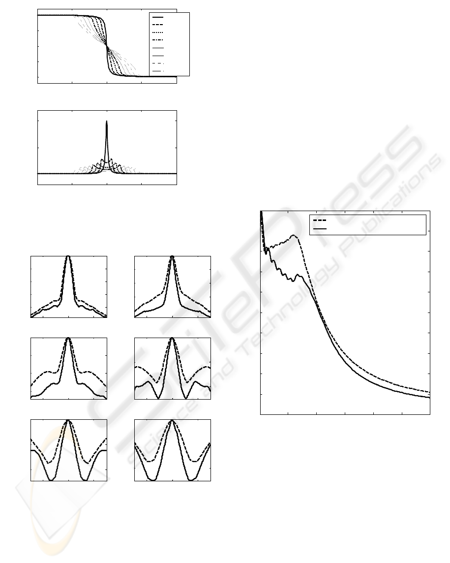
Figure 1: Voltage excitations to approximate beamforming
of the 0-order X wave in: a) pressure, b) velocity potential.
-20 0 20
0.2
0.4
0.6
0.8
a) z=100 mm
-20 0 20
0.2
0.4
0.6
0.8
b) z=200 mm
-20 0 20
0.4
0.6
0.8
1
c) z=300 mm
-20 0 20
0.6
0.8
1
d) z=400 mm
-20 0 20
0.6
0.8
1
e) z=500 mm
Amplitude normalized
-20 0 20
0.6
0.8
1
f) z=600 mm
Lateral axis X [mm]
Figure 2: Normalized lateral axis 1-D profiles with regard
to the maximum in each case, for two beam-forming
approximations using the 0-order X wave expressions in
pressure and velocity potential. The figure shows the beam
profiles resulting in the pressure field, emitted by an
ultrasonic annular array of 8-rings, for the case of using
the X wave in pressure (dash line) and the X wave in
velocity potential (continue line).
The figure 2 shows the lateral axis pressure profiles
for the 0-order X waves expressed in pressure and
velocity potential, in both cases in one dimension (1-
D) and for distinct depths between 100 and 500 mm.
In this figure, it is clearly show that for the case of
using the expression of the velocity potential, the
resulting sidelobes, from depths superior to 100mm,
are quite smaller than in the case of using the
pressure expression.
The figure 3 shows the axial pressure profiles
normalized with regard to the maximum in both
cases (driving derived from
pressure and velocity
potential expressions)
. In this figure, the case of using
the X wave in pressure shows more uniform field
amplitude, and in addition, the case of using the X
wave in velocity potential originates a field decay
with a certain ringing.
100 200 300 400 500 600
0
0.1
0.2
0.3
0.4
0.5
0.6
0.7
0.8
0.9
1
Axial axis Z [mm]
Amplitude normalized
Axial profile for x=0 mm
X wave in pressure
X wave in velocity potential
Figure 3: Morphology of axial pressure profiles
normalized with regard to the maximum in each case, by
approximating the beam-forming from the 0-order X
waves in pressure (dash line), and velocity potential
(continue line).
In relation to two-dimensional (2-D) field displays,
figure 4 shows the spatial x-z distribution of the
maxima amplitudes of the envelopes of the pressure
field, normalized with regard to the display
maximum in the two alternative cases (X wave
expressions formulated in pressure and velocity
potential terms). This figure shows that the pressure
field when using for calculation the X wave in
pressure is more stable than in the case of using the
velocity potential. Furthermore, the case of using the
SYNTHESIS OF DRIVING SIGNALS FOR MEDICAL IMAGING ANNULAR ARRAYS FROM ULTRASONIC
X-WAVE SOLUTIONS
293
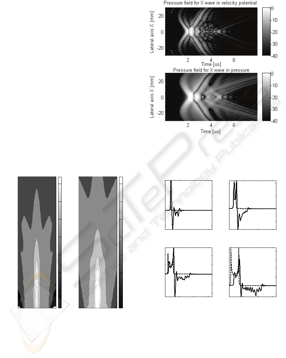
X wave in velocity potential produces a field with a
narrower beamwidth and approximately with the
same depth of field (measured at -6 dB) that when
using pressure X wave, but showing some axial field
ringing, with two discontinuous regions appearing in
the -3 dB contour curve. This field ringing is due to
the especial behaviour of the positive and negative
regions in the pressure field signals (see figure 7).
And the figure 5 shows other type of 2-D display
(space-temporal) of beamforming results by using
the 0-order X waves in terms of pressure, and
velocity potential, particularized for z = 100 mm,
just a depth very usual in abdominal and cardiologic
medical imaging. The resulting ultrasonic beam in
this case, when the X wave expression in velocity
potential is used, has two principal field maxima at
the beginning of time axis, and some smaller
secondary peaks afterwards, because of the strong
diffraction effects in this zone. And, the case of
using the X wave expression in pressure shows only
one main maximum also with some secondary
peaks, originated by the phenomenon of diffraction.
-20 0 20
50
100
150
200
250
300
350
400
450
500
550
Lateral axis X [mm]
Axial axis Z [mm]
X wave in velocity potential
-20 0 20
50
100
150
200
250
300
350
400
450
500
550
Lateral axis X [mm]
X wave in pressure
-40
-35
-30
-25
-20
-15
-10
-5
-40
-35
-30
-25
-20
-15
-10
-5
Figure 4: 2-D Display of the signal envelopes maxima in
the pressure field, normalized with regard to the maximum
in each case, for beam-forming approximation from the 0-
order X waves in pressure and in velocity potential. The
shown slices are in: -3 dB, -6 dB, -12 dB, -20 dB, -40 dB.
Figures 6-7 show waveforms in points of the x axis,
obtained by a beamforming using 0-order X waves:
in pressure and velocity potential.
Figure 5: Pressure fields in spatial-temporal distribution,
normalized with regard to the maximum in each 2-D
display, by using 0-order X waves in pressure and velocity
potential. The pressure field levels are shown in grey scale
detailed in dB, for the axial distance z = 100 mm.
0 0.5 1 1.5
x 10
-5
-0.5
0
0.5
1
a) x = 0 mm
Tim e [ s]
Normalized amplitude
0 0.5 1 1.5
x 10
-5
-0.1
0
0.1
0.2
b) x = 10 mm
Time [ s]
Normalized amplitude
0 0.5 1 1.5
x 10
-5
-0.1
-0.05
0
0.05
0.1
c) x = 20 mm
Tim e [ s]
Normalized amplitude
0 0.5 1 1.5
x 10
-5
-0.02
0
0.02
0.04
0.06
0.08
d) x = 30 mm
Time [ s]
Normalized amplitude
Figure 6: Pressure signal waveforms in x axis, at z = 100
mm, obtained with an annular array of 8-rings, normalized
with regard to maximum, for beam-forming using the 0-
order X wave in pressure (continue line) and the
theoretical pressure field signals for X wave in pressure
(dashes line).
BIOSIGNALS 2010 - International Conference on Bio-inspired Systems and Signal Processing
294
0 0.5 1 1.5
x 10
-5
-0.5
0
0.5
1
Time [s ]
Normalized amplitude
a) x = 0 mm
0 0.5 1 1.5
x 10
-5
-0.2
-0.1
0
0.1
Tim e [ s]
Normalized amplitude
b) x = 10 mm
0 0.5 1 1.5
x 10
-5
-0.15
-0.1
-0.05
0
0.05
Time [s ]
Normalized amplitude
c) x = 20 mm
0 0.5 1 1.5
x 10
-5
-0.05
0
0.05
Tim e [ s]
Normalized amplitude
d) x = 30 mm
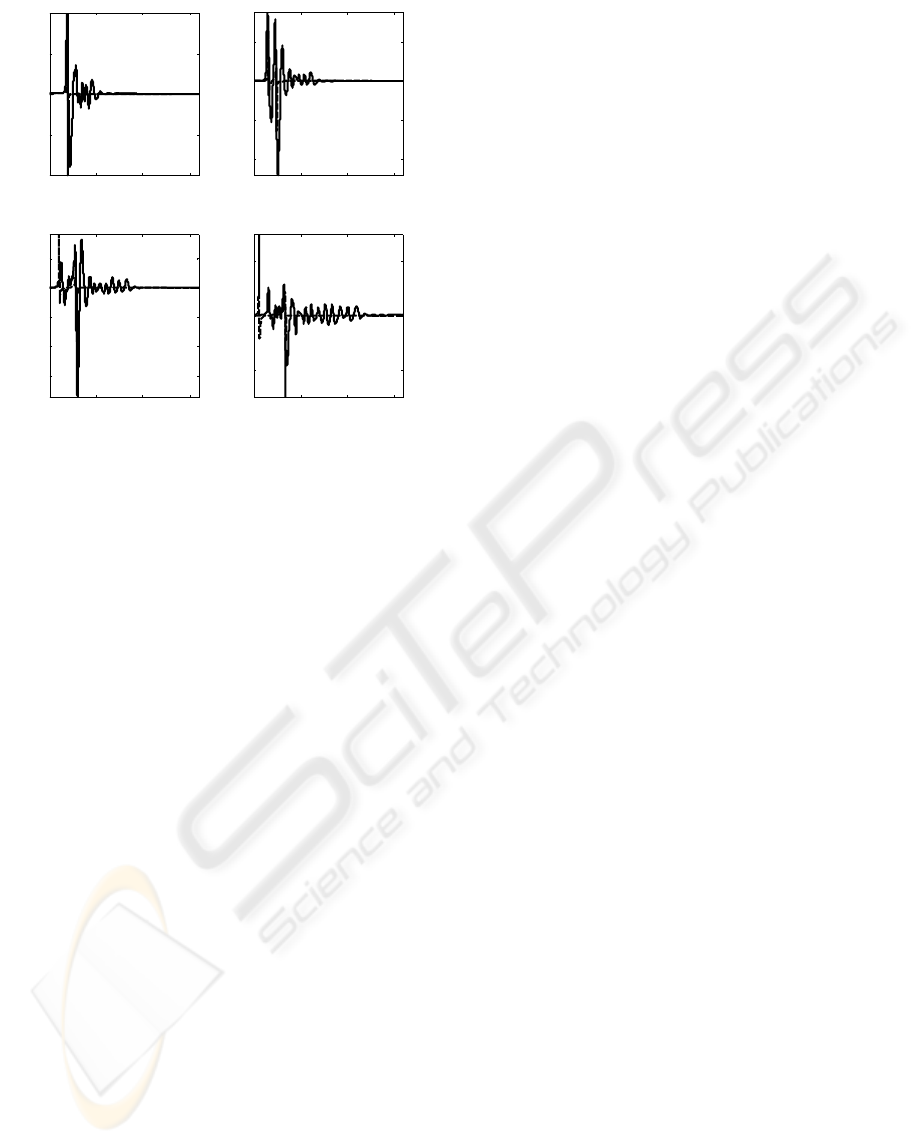
Figure 7: Pressure signal waveforms in x axis, at z = 100
mm, obtained with an annular array of 8-rings, normalized
with regard to maximum, for beam-forming using the 0-
order X wave in velocity potential (continue line), and
theoretical pressure field signals for X wave in pressure
(dashes line).
These figure show the time pressure signals for 4
points in the x axis, at a depth of z = 100 mm,
obtained with an annular array of 8-rings, and the
different signals are normalized with regard to the
maxima signal amplitude. They show the similarity
of signals morphology with the theoretical pattern
for pressure field signals.
3 CONCLUSIONS
Results suggest that the procedure proposed in this
paper by inverse processing from X-waves, as a tool
for ultrasonic beam-forming analysis, creates new
beam collimation options in high resolution medical
imaging, constitutes a very useful and promising
way to generate and evaluate beams alternatives to
those derived from classical proposals to generate X-
wave field distributions. And it could be also used
for synthesizing special excitations of annular arrays
to create other type of limited diffraction beams.
The good performance of the options evaluated
here for beam focusing along certain field depths,
potentiality confirms the suitability of the proposed
tool. It seems also possible a successful application
of it to synthesize the multiple driving needed for
creating other types of high-resolution ultrasonic
beams, also in terms of pressure, for future advanced
bio-medical imaging equipment. As future work, it
would be of quite interest, studying the effects of the
ring widths, in the annular array, over the resulting
beam properties, in order to optimize the
morphology of the signals and of the field spatial
distributions, and also to achieve a further reduction
of the diffraction effects.
ACKNOWLEDGEMENTS
This work and the grant of Eng. L. Castellanos in
CSIC (Videus lab) are being supported by the R&D
National Plan of the Spanish Minister ‘‘Science &
Innovation” ( Projects: PN-DPI2005-00124 and PN-
DPI2008-05213 ). The scientific stay of Dr. H. Calás
in the Dpt. SSTU of the Acoustic Institute in Madrid
is supported by Post-doctoral JAE Program (CSIC).
REFERENCES
Arnau, A., “Piezoelectric Transducer and Aplications”,
Edit. Springer, ISBN 3-540-20998-0, 2004.
Crespo., Y., Calas H., Moreno E., Eiras J. A., Secada J.
D., Leija L., “New X-wave solutions of
isotropic/homogenous scalar wave equation”, ICEEE
and CIE, IEEE Catalog Number: 05EX1097, ISBN: 0-
7803-9230-2, p. 164-167, 2005.
Donnelly, R., Ziolkowski R., “A method for constructing
solutions of homogeneous partial differential
equations: localized waves”, Proc. R. Soc. Lond. A.,
No. 437, p. 673-692, 1992.
Lu, J. Y., Greenleaf, J. F., “Theory and Acoustic
Experiments of Nondiffracting X Waves”, IEEE
Ultrason. Symp. Proc., p. 1155, 1991.
Mason, W. P., “Physical Acoustics, Volume I-Part A”,
Edit. Academic Press, 1964.
Püttmer, A., Hauptmannm P., Lucklum, R., Krause, O.,
Henning B., “SPICE model for lossy piezoceramic
transducer”, IEEE Trans. Ultrason. Ferroelec. Freq.
Contr., Vol. 44, No. 1, p. 60-66, 1997.
Stepanishen, P. R., “Transient radiation from pistons in an
infinite planar baffle”, J. Acoust. Soc. Am., Vol. 49
(5B), p. 1629, 1971.
Strutt, J. W., “The Theory of Sound”, Vol. 2, Edit.
MacMillian & Co., Second Edition, 1896.
Sushilov, Nikolai V., Tavakkoli, J., Cobbold R. S. C.,
“New X-wave solutions of free-space scalar wave
equation and their finite size realization”, IEEE
Transactions on Ultrasonics, Ferroelectrics, and
Frequency Control, Vol. 48, No. 1, p. 274-284, 2001.
Ullate, L. G., Ramos, A., San Emeterio, J. L., “Analysis of
the ultrasonic field radiated by time – delay
cylindrically focused linear arrays”. IEEE Trans.
Ultrason. Ferroelec. Freq. Control., Vol. 41, nº 5, p.
749-760, 1994.
SYNTHESIS OF DRIVING SIGNALS FOR MEDICAL IMAGING ANNULAR ARRAYS FROM ULTRASONIC
X-WAVE SOLUTIONS
295
