
DISCO
VERING N-ARY TIMED RELATIONS FROM SEQUENCES
Nabil Benayadi and Marc Le Goc
LSIS Laboratory, University Saint Jerome, Marseille, France
Keywords:
Markov Chain, Information Theory, Kullback-Leibler Distance.
Abstract:
The goal of this position paper is to show the problems with most used timed data mining techniques for dis-
covering temporal knowledge from a set of timed messages sequences. We will present from a simple example
that Apriori-like algorithms for mining sequences as Minepi and Winepi fail for mining a simple sequence
generated by a very simple process. Consequently, they cannot be applied to mine sequences generated by
complexes process as blast furnace process. We will show also that another technique called TOM4L(Timed
Observations Mining for Learning) can be used for mining such sequences and generate significantly better
results than produced by Apriori-like techniques. The results obtained with an application on very complex
real world system is presented to show the operational character of the TOM4L.
1 INTRODUCTION
When supervising and monitoring dynamic pro-
cesses, a very large amount of timed messages
(alarms or simple records) are generated and collected
in databases. Mining these databases allows discov-
ering the underlying relations between the variables
that govern the dynamic of the process.
Apriori-like techniques (Roddick and
Spiliopoulou, 2002) are probably the most used
methods for discovering temporal knowledge in
timed messages sequences. The basic principle of
these approaches uses a representativeness criterion;
typically the support to build the minimal set of
sequential patterns that describes the given set of
sequences. The support s(p
i
) of a pattern p
i
is
the number of sequences in the set of sequences
where the pattern p
i
is observed. A frequent pattern
is a pattern p
i
with a support s(p
i
) greater than a
user defined thresholds S, s(p
i
) ≥ S. A frequent
pattern is interpreted as a regularity or a condensed
representation of the given set of sequences.
The Timed Data Mining techniques differ depend-
ing on whether the initial set of sequences is a single-
ton or not. The second case is the simpler because
the decision criterion based on the support is directly
applicable to a set of sequences. When the initial set
of sequences contains a unique sequence, the notion
of windows has been introduced to define an adapted
notion of support. The first way consists in defining
a fixed size of windows that an algorithm like Winepi
(Mannila et al., 1997) shifts along the sequence: the
sequence becomes then a set of equal length sub-
sequences and the support s(p
i
) of a pattern can be
computed. The second way consists in building a win-
dow for an a priori given pattern p
i
. With the Minepi
algorithm for example (Mannila et al., 1997), a win-
dow W = [t
s
,t
e
[ is a minimal occurrence of p
i
if p
i
occurs in W and not in any sub-window of W . In
practice, a maximal window size parameter maxwin
must be defined to bound the search space of pat-
terns. Unfortunately, these approaches present two
main problems. The first is that the algorithms require
the setting of a set of parameters: the discovered pat-
terns depends therefore of the tuning of the algorithms
(Mannila, 2002). The second problem is the number
of generated patterns that is not linear with threshold
value S of the decision criterion s(p
i
) ≥ S. In prac-
tice, to obtain an interesting set of frequent pattern, S
must be small. Consequently, the number of frequent
is huge. Practically, only a very small fraction of the
discovered patterns are interesting.
We will show in this paper that the TOM4L ap-
proach (Bouch
´
e, 2005; Le Goc, 2006) can avoid these
two problems with the use of a stochastic representa-
tion of a given set of sequences on which an inductive
reasoning coupled with a deductive reasoning is ap-
plied to reduce the space search.
The next section presents a (very) simple illus-
trative example and shows these two main problems
428
Benayadi N. and Le Goc M. (2010).
DISCOVERING N-ARY TIMED RELATIONS FROM SEQUENCES.
In Proceedings of the 2nd International Conference on Agents and Artificial Intelligence - Artificial Intelligence, pages 428-433
DOI: 10.5220/0002762304280433
Copyright
c
SciTePress

for the most used algorithms for discovering temporal
knowledge in timed messages sequences, Winepi and
Minepi algorithms. Next, section 3 introduces the ba-
sis of the TOM4L process and the section 4 describes
the results obtained with an application of the TOM4L
on very complex real system monitored with a large
scale knowledge based system, the Sachem system of
the Arcelor-Mittal Steel group. Section 5 concludes
the paper.
2 AN ILLUSTRATIVE EXAMPLE
The illustrative example is a simple dynamic SISO
(Single Input Single Output) system y(t) = F · x(t)
where F is a convolution operator. This example is
used through this paper to illustrate the claims.
Let us defining two thresholds ψ
x
and ψ
y
for the input
variable x(t) and the output variable y(t). These two
thresholds respectively define two ranges for each of
the variables: rx
0
=] − ∞, ψ
x
], rx
1
=]ψ
x
, +∞], ry
0
=
] − ∞, ψ
y
] and ry
1
=]ψ
y
, +∞]). Let us suppose that
there exists a (very simple) program that writes a con-
stant when a signal enter in a range. Such a pro-
gram writes the constant 1 (resp. H) when x(t) (resp.
y(t)) enters in the range rx
1
(resp. ry
1
) and 0 (resp.
L) when x(t) (resp. y(t)) enters in the range rx
0
(resp. ry
0
). The evolution of the x(t) in the figure
1 leads to the following sequence: Ω = {(1,t
1
), (H, t
2
),
(0,t
3
), (L,t
4
), (1,t
5
), (H,t
6
), (0,t
7
), (L,t
8
), (1,t
9
), (H,t
10
),
(0,t
11
), (L, t
12
), (1, t
13
), (H, t
14
), (0, t
15
), (L, t
16
), (1, t
17
),
(H, t
18
), (0,t
19
), (L,t
20
), (1,t
21
), (H,t
22
), (0,t
23
), (L,t
24
)}.
x(t)
t
y(t)
t
ω
1
ω
0
1 3 5 7 9 11 13 15 17 19 21 23
t
ω
H
ω
L
2 4 5 8 10 12 14 16 18 20 22 24
t
x
y
1
0
H
L
Figure 1: Temporal evolution of variables x and y.
To illustrate the sensitivity of the Winepi and the
Minepi algorithms to the parameters, we define two
sets of parameters and apply the algorithms to the se-
quence Ω. In the first set of parameters, the window
width w and window movement v for Winepi are both
set to 4 (this is the ideal tuning) and for Minepi, the
max window is set to 4 and the minimal frequency is
fixed to 6 (this is also the ideal tuning). In the sec-
ond set of parameters, the window width and window
movement of Winepi are equal to 8 and the support
is equal to 3. The minimal frequency for Minepi is
set to 8. The table 1 provides the number of patterns
discovered by each algorithm with the two sets of pa-
rameters.
These two experimentation show the sensitivity of
the Winepi and the Minepi algorithms with the param-
eters: from the first set to the second, the number of
patterns increases of more than 626% for Winepi, and
more than 18666% from Minepi. The main problem
is the too large number of discovered patterns. The
paradox is then the following: to find the ideal set of
parameters that minimizes the number of discovered
patterns, the user must know the system while this
is precisely the global aim of the Data Mining tech-
niques. There is then a crucial need for another type
of approach that is able to provide a good solution for
such a simple system and provide operational solu-
tions for real world systems. The aim of this paper
is to propose such an approach: the TOM4L process
(Timed Observation Mining for Learning) finds only
four relations with the example without any parame-
ters.
Table 1: Number of Discovered Patterns.
Winepi Minepi
First parameter set 15 15
Second parameter set 94 2800
3 BASIS OF THE TOM4L
PROCESS
The TOM4L process is based on the Theory of Timed
Observations of (Le Goc, 2006) that provides the
mathematical foundations of the four steps Timed
Data Mining process that reverses the usual Data Min-
ing process in order to minimize the size of the set of
the discovered patterns:
1. Stochastic Representation of a set of sequences
Ω = {ω
i
}. This step produces a set of timed bi-
nary relations of the form R
i, j
(C
i
,C
j
, [τ
−
i, j
, τ
+
i, j
]).
2. Induction of a minimal set of timed binary rela-
tions. This step uses an interestingness criterion
based on the BJ-measure describes in the follow-
ing section.
3. Deduction of a minimal set of n-ary relations.
This step uses an abductive reasoning to build a
set of n-ary relations that have some interest ac-
cording to a particular problem.
4. Find the minimal set of n-ary relations being rep-
resentatives according to the problem. This step
corresponds to the usual search step of sequential
patterns in a set of sequences in Minepi or Winepi.
DISCOVERING N-ARY TIMED RELATIONS FROM SEQUENCES
429

The discovered n-ary relations discovered in the last
step are called signatures. The next section provides
the basic definitions of the Timed Observations The-
ory.
3.1 Basic Definitions (Le Goc, 2006)
A discrete event e
i
is a couple (x
i
, δ
i
) where x
i
is the
name of a variable and δ
i
is a constant. The constant
δ
i
denotes an abstract value that can be assigned to the
variable x
i
. The illustrative example allows the defini-
tion of a set E of four discrete events: E = {e
1
≡ (x, 1),
e
2
≡ (x, 0), e
3
≡ (y, H), e
4
≡ (y, L)}. A discrete event
class C
i
= {e
i
} is an arbitrary set of discrete event
e
i
= (x
i
, δ
i
). Generally, and this will be true in the
suite of the paper, the discrete event classes are de-
fined as singletons because when the constants δ
i
are
independent, two discrete event classes C
i
= {(x
i
, δ
i
)}
and C
j
= {(x
j
, δ
j
)} are only linked with the variables x
i
and x
j
. The illustrative example allows the definition
of a set Cl of four discrete event classes: Cl = {C
1
=
{e
1
}, C
0
= {e
0
}, C
L
= {e
L
}, C
H
= {e
H
}}.
An occurrence o(k) of a discrete event class C
i
= {e
i
},
e
i
= (x
i
, δ
i
), is a triple (x
i
, δ
i
,t
k
) where t
k
is the time
of the occurrence. When useful, the rewriting rule
o(k) ≡ (x
i
, δ
i
,t
k
) ≡ C
i
(k) will be used in the follow-
ing. A sequence Ω = {o(k)}
k=1...n
, is an ordered set
of n occurrences C
i
(k) ≡ (x
i
, δ
i
,t
k
). The illustrative ex-
ample defines the following sequence: Ω = {(C
1
(1),
C
H
(2), C
0
(3), C
L
(4), C
1
(5), C
H
(6), C
0
(7), C
L
(8), C
1
(9),
C
H
(10), C
0
(11), C
L
(12), C
1
(13), C
H
(14), C
0
(15), C
L
(16),
C
1
(17), C
H
(18), C
0
(19), C
L
(20), C
1
(21), C
H
(22), C
0
(23),
C
L
(24)}.
Le Goc (Le Goc, 2006) shows that when the con-
stants δ
i
∈ ∆ are independent, a sequence Ω = {o(k)}
defining a set Cl = {C
i
} of m classes is the superposi-
tion of m sequences ω
i
= {C
i
(k)}:
Ω = {o(k)} =
[
i=1...m
ω
i
= {C
i
(k)} (1)
The Ω sequence of the illustrative example is then
the superposition of four sequences ω
i
= {C
i
(k)}:
ω
1
= {C
1
(1),C
1
(5),C
1
(9),C
1
(13),C
1
(17),C
1
(21)}
ω
0
= {C
0
(3),C
0
(7),C
0
(11),C
0
(15),C
0
(19),C
0
(23)}
ω
L
= {C
L
(4),C
L
(8),C
L
(12),C
L
(16),C
L
(20),C
L
(24)}
ω
H
= {C
H
(2),C
H
(6),C
H
(10),C
H
(14),C
H
(18),C
H
(22)}
3.2 Stochastic Representation
The stochastic representation transforms a set of se-
quences ω
i
= {o(k)} in a Markov chain X = (X(t
k
);k >
0) where the state space Q = {q
i
}, i = 1 . . . m, of X
is confused with the set of m classes Cl = {C
i
} of
Ω =
[
i
ω
i
.
Consequently, two successive occurrences (C
i
(k −
1), C
j
(k)) correspond to a state transition in X:
X(t
k−1
) = q
i
−→ X(t
k
) = q
j
. The conditional proba-
bility P
£
X(t
k
) = q
j
|X(t
k−1
) = q
i
¤
of the transition from
a state q
i
to a state q
j
in X corresponds then to the
conditional probability P
£
C
j
(k) ∈ Ω|C
i
(k − 1) ∈ Ω
¤
of
observing an occurrence of the class C
j
at time t
k
knowing that an occurrence of a class C
i
at time t
k−1
has been observed: The transition probability matrix
P = [p
i, j
] of X is computed from the contingency ta-
ble N = [n
i, j
], where n
i, j
∈ N is the number of couples
(C
i
(k),C
j
(k + 1)) in Ω. For example, the table 2 is
the contingency table N of the sequence Ω of the il-
lustrative example.
Table 2: Contingency table N = [n
i, j
] of Ω.
C
1
C
0
C
H
C
L
Total
C
1
0 0 6 0 6
C
0
0 0 0 6 6
C
H
0 6 0 0 6
C
L
5 0 0 0 5
Total 5 6 6 6 23
The stochastic representation of a given set Ω
of sequences is then the definition of a set R =
{R
i, j
(C
i
,C
j
, [τ
−
i j
, τ
+
i j
])} where each the conditional prob-
ability p
i, j
= P
£
C
j
(k) ∈ Ω|C
i
(k − 1) ∈ Ω
¤
of each binary
relation R
i, j
(C
i
,C
j
, [τ
−
i j
, τ
+
i j
]) is not null. The timed con-
strains [τ
−
i j
, τ
+
i j
] is provided by a function of the set D
of delays D = {d
i j
} = {(t
k
j
− t
k
j
)} computed from the
binary superposition of the sequences ω
i, j
= ω
i
∪ ω
j
:
τ
−
i j
= f
−
(D), τ
+
i j
= f
+
(D). For example, the authors of
(Bouch
´
e, 2005) use the properties of the Poisson law
to compute the timed constraints: τ
−
i j
= 0, τ
+
i j
=
1
λ
i, j
where λ
i, j
is the Poisson rate (the exponential inten-
sity) of the exponential law that is the average delay
d
i j
moy
=
∑
(d
i j
)
Card(D)
.
The set R of the illustrative example is the following:
R = {R
1,H
(C
1
,C
H
, [τ
−
1,H
, τ
+
1,H
]), R
0,L
(C
0
,C
L
, [τ
−
0,L
, τ
+
0,L
]),
R
H,0
(C
H
,C
0
, [τ
−
H,0
, τ
+
H,0
]), R
L,1
(C
L
,C
1
, [τ
−
L,1
, τ
+
L,1
])}.
3.3 Induction of Binary Relations
The induction step in TOM4L consists to select a sub-
set I of R, I ⊆ R, where each relation R
i, j
(C
i
,C
j
)
in I presents a potential interest. This selection is
based on the definition of an interestingness measure
of temporal binary relation R
i, j
(C
i
,C
j
), called BJ-
Measure. The BJ-Measure of timed binary relation
R
i, j
(C
i
,C
j
) is the adaptation of the kullback-Leibler
distance to timed data (Benayadi and Goc, 2008). The
BJ-Measure evaluates the information amount car-
ICAART 2010 - 2nd International Conference on Agents and Artificial Intelligence
430

ried by an observation of the class C
i
to an obser-
vation of the class C
j
. The principle of this adap-
tation is to consider the set of n binary relations as
set of binary communication channels without mem-
ory (in the sense of Shannon, see Figure 2). Each
binary relation R
i, j
(C
i
,C
j
) ∈ R is represented by a dis-
crete binary memoryless channel linking two abstract
binary variables X and Y , where X(t
k
) ∈ {C
i
,C
i
} and
Y (t
k+1
) ∈ {C
j
,C
j
}. The class C
i
(resp. C
j
) represents
all classes in Cl except C
i
: Cl − C
i
(resp. Cl − C
j
)
where its occurrence number is the average of occur-
rence number of each classes in C
i
(resp. C
j
). There-
fore, any sequence (C
i
(k),C
j
(k + 1)) ∈ Ω is an exam-
ple of R
i, j
(C
i
,C
j
) and each (C
i
(k),C
j
(k + 1)) ∈ Ω or
(C
i
(k),C
j
(k + 1)) ∈ Ω is counter-example.
Two adaptations of Kullback-Liebler distance are pro-
posed to calculate the interestingness of the binary
relation R
i, j
(C
i
,C
j
) ∈ R, the first is from the point of
view of class C
i
, the BJ-measure in length, the other
is from the point of view of C
j
, the BJ-measure in
width. The BJ-measure in length of a binary rela-
tion R
i, j
(C
i
,C
j
) ∈ R, noted BJL(C
i
,C
j
), measures the
amount of information provided by an occurrence of
the class C
i
on an occurrence of class C
j
or class C
j
:
• if p( j|i) ≥ p( j) then BJL(C
i
,C
j
) = D(p(Y |C
i
)kp(Y ))
• else BJL(C
i
,C
j
) = 0
Figure 2: Two abstract binary variables connected by a dis-
crete memoryless channel.
Symmetrically, the BJ-measure in width of a bi-
nary relation R
i, j
(C
i
,C
j
) ∈ R, noted BJW (C
i
,C
j
), mea-
sures the amount of information provided by an oc-
currence of the class C
i
or C
i
on an occurrence of
the class C
j
. The values of both measures are high
when the informational contribution of the class C
i
on C
j
is strong. To have a global vision of the infor-
mational contribution of the class C
i
on C
j
, the two
measures are combined into a single measure noted
M. The measure M is simply the norm of the vector
µ
BJL(C
i
,C
j
)
BJW (C
i
,C
j
)
normalized between 0 and 1.
For example, the values of the M-measure of the set
R = {R
1,H
(C
1
,C
H
, [τ
−
1,H
, τ
+
1,H
]), R
0,L
(C
0
,C
L
, [τ
−
0,L
, τ
+
0,L
]),
R
H,0
(C
H
,C
0
, [τ
−
H,0
, τ
+
H,0
]), R
L,1
(C
L
,C
1
, [τ
−
L,1
, τ
+
L,1
])} of the
illustrative example are given in table 3.
Table 3: Matrix M.
C
1
C
0
C
H
C
L
C
1
0 0 1 0
C
0
0 0 0 1
C
H
0 1 0 0
C
L
1 0 0 0
Table 4: The M values evolution with different λ
err
.
λ
err
R(C
1
,C
H
) R(C
H
,C
0
) R(C
0
,C
L
) R(C
L
,C
1
)
0 1 1 1 1
6 0.75 0.56 1 0.63
12 0.78 0 1 0
18 0.61 0 0.79 0
24 0.55 0 0.55 0
30 0 0 0 0
In this example, the relations
R
1,H
(C
1
,C
H
, [τ
−
1,H
, τ
+
1,H
]) and R
0,L
(C
0
,C
L
, [τ
−
0,L
, τ
+
0,L
])
have not the same meaning as the relations
R
H,0
(C
H
,C
0
, [τ
−
H,0
, τ
+
H,0
]) R
L,1
(C
L
,C
1
, [τ
−
L,1
, τ
+
L,1
]):
only the two first are linked with the system
y(t) = Fx(t), the two latters being only sequential
relation (the system computes the values of y(t), not
the values of x(t)).
To distinguish between these two kinds of rela-
tions, the idea in the induction step is to add noise
in the initial set of sequences. To this aim, we de-
fined the ”noisy” observation class C
err
the occur-
rences of which are randomly timed. If a relation
R
i, j
(C
i
,C
j
, [τ
−
i, j
, τ
+
i, j
]) is a property of the system, then
the time interval between the occurrences of the C
i
and C
j
classes will be more regular than if this re-
lation is a purely sequential relation. The table 4
shows the values of the M-measures of the relations
R(C
1
,C
H
), R(C
H
,C
0
), R(C
0
,C
L
) and R(C
L
,C
1
) with dif-
ferent rate λ
err
=
n
err
t
24
−t
0
of noisy occurrences added
in Ω. The table 4 shows that when λ
err
∈ { 12, 24}, the
binary relations R(C
H
,C
0
) and R(C
L
,C
1
) disappears.
Naturally, when the noise is too strong (λ
err
= 30), all
the relations disappear: this means that at least one
occurrence C
err
(k) is systematically inserted between
two occurrences of the initial sequence Ω.
This example leads also to an operational property of
the M-measure: when θ
i, j
À 1 or θ
i, j
¿ 1, one class
plays the same role of a noisy class for the other. This
situation arises in the two following cases:
• n
i, j
≥ n
i, j
⇒ p( j|i) ≥ 0.5. The C
j
plays the role
of a noisy class for the class C
i
.
DISCOVERING N-ARY TIMED RELATIONS FROM SEQUENCES
431

• n
i, j
≥ n
i, j
⇒ p( j|i) ≥ 0.5. The C
i
plays the role of
a noisy class for the class C
j
.
These two conditions are both evaluated when
comparing the product p( j|i) · p(i| j) with
1
2
·
1
2
: when
p( j|i) · p(i| j) ≤
1
4
, M(C
i
,C
j
) ≤ 0.5 and the relation
R
i, j
(C
i
,C
j
) cannot be justified with the M-measure.
Inversely, when p( j|i) · p(i| j) >
1
4
, M(C
i
,C
j
) > 0.5
and the relation R
i, j
(C
i
,C
j
) has some interest from the
point of view of the M-measure. This leads to the fol-
lowing simple inducing rule that uses the M-measure
as interestingness criteria:
M(C
i
,C
j
) > 0.5 ⇒ R
i, j
(C
i
,C
j
) ∈ I (2)
So, the set I of induced binary relations contains only
two binary relations : I = {R
1,H
(C
1
,C
H
, [τ
−
1,H
, τ
+
1,H
]),
R
0,L
(C
0
,C
L
, [τ
−
0,L
, τ
+
0,L
])}
3.4 Deduction of n-ary Relations
The set I of binary relations contains then the minimal
subset of R where each relation R
i, j
(C
i
,C
j
) presents
a potential interest. From this set, the objective of
the deduction step consists to deduce from I a small
set M = {m
k−1,n
} of n-ary relations m
k−1,n
so that
a search algorithm can be used effectively to iden-
tify the most representative relations m
k−1,n
. To this
aim, an heuristic h(m
i,n
) is to select a minimal set
M = {m
k,n
} of n-ary relations of the form m
k,n
=
{R
i,i+1
(C
i
,C
i+1
)}, i = k, ··· , n− 1, that is to say paths
leading to a particular final observation class C
n
. The
heuristic h(m
i,n
) makes a compromise between the
generality and the quality of a path m
i,n
:
h(m
i,n
) = card(m
i,n
) × BJL(m
i,n
) × P(m
i,n
) (3)
In this equation, card(m
i,n
) is the number of relations
in m
i,n
, BJL(m
i,n
) is the sum of the BJL-measures
BJL(C
k−1
,C
k
) of each relation R
k−1,k
(C
k−1
,C
k
) in
m
i,n
and P(m
i,n
) is the product of the probabilities as-
sociated with each relation in m
i,n
.
P(m
i,n
) corresponds to the Chapmann-
Kolmogorov probability of a path in the transition
matrix P = [p(k − 1, k)] of the Stochastic Represen-
tation. The interestingness heuristic h(m
i,n
) being
of the form φ · ln(φ), it can be used to build all the
paths m
i,n
where h(m
i,n
) is maximum (Benayadi and
Le Goc, 2008). For the illustrative example, the
deduction step found a set M of two binary relations
(M = I)
1
.
1
no paths containing more than one binary relation can
be deduced from I
Cover Rate
number of target class occurrences predicted by the model
Total number of target class occurrences
Anticipation Rate
TP
TP FP
TP True Positive Prediction
FP False Positive Prediction
Figure 3: Evaluation Measures for n-ary relation.
3.5 Find Representativeness n-ary
Relations
Given a set M = {m
k,n
)} of paths m
k,n
=
{R
i,i+1
(C
i
,C
i+1
)}, i = k, · ·· , n − 1, the fourth and
final step of the discovery process TOM4L, step Find,
uses two representativeness criterion (Cover Rate
and Anticipation Rate, figure 3) to build the subset
S ⊆ M containing the pathes m
k,n
being representative
according the initial set Ω of sequences. These paths
are called Signatures.
Generally, a threshold equal to 50% is used to
discard n-ary relations which have more false pre-
diction than correct prediction. For example, the
values of the cover rate and the anticipation rate of
both binary relations of M of the illustrative example
are 100%. So, S = M, S = {R
1,H
(C
1
,C
H
, [τ
−
1,H
, τ
+
1,H
]),
R
0,L
(C
0
,C
L
, [τ
−
0,L
, τ
+
0,L
])}.
These signatures are the only relations (patterns) that
are linked with the system y(t) = Fx(t). Compar-
ing with the set of patterns found by Apriori-like ap-
proaches, we can confirm from this illustrative ex-
ample that TOM4L approach converges towards a
minimal set of operational relations, which describe
the dynamic of the process. In the next section, we
present the application of TOM4L on a sequence gen-
erated by a very complex dynamic process, blast fur-
nace process. Due to the process complexity, we
can confirm, without experience, that Apriori-like ap-
proaches fail to mine this sequence.
4 APPLICATION
Our approach has been applied to sequences gener-
ated by knowledge-based system SACHEM devel-
oped to monitor, diagnose and control the blast fur-
nace (Le Goc, 2006). We are interested with the
omega variable that reveals the wrong management
of the whole blast furnace. The studied sequence
comes from Sachem at Fos-Sur-Mer (France) from
08/01/2001 to 31/12/2001. It contains 7682 occur-
rences of 45 discrete event classes (i.e. phenomena).
For the 1463 class linked to the omega variable, the
search space contains about 20
5
= 3, 200, 000 binary
relations. The inductive and the abductive reasoning
ICAART 2010 - 2nd International Conference on Agents and Artificial Intelligence
432
steps of TOM4L produces a minimal set M of only
166 binary relations from which the set S of signa-
tures of figure 5 have been discovered (Ta = 50% and
T c = 10%). The set S is made with 50 binary rela-
tions.
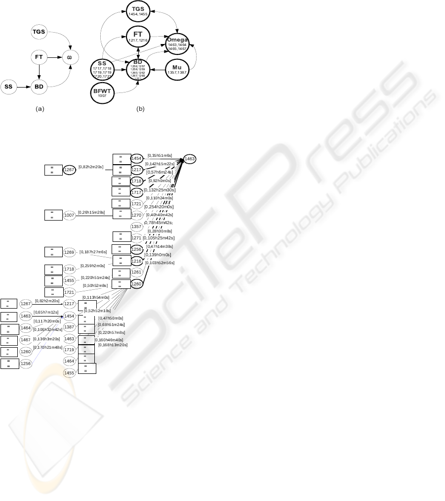
ω
Figure 4: Expert’s (1995, a) and discovered relations (2007,
b).
Ta 62 %
Tc 74 %
Ta 58 %
Tc 53 %
Ta 62 %
Tc 14 %
Ta 156%
Tc 26 %
Ta 100 %
Tc 22 %
Ta 257 %
Tc 14 %
Ta 62 %
Tc 37 %
Ta 56 %
Tc 24 %
Ta 133 %
Tc 42 %
Ta 73 %
Tc 13 %
Ta 55 %
Tc 12 %
Ta 50 %
Tc 13 %
Ta 141%
Tc 45 %
Ta 119 %
Tc 51 %
Ta 88 %
Tc 19 %
Ta 88 %
Tc 19 %
Ta 88 %
Tc 30 %
Ta 105%
Tc 15 %
Ta 102 %
Tc 36 %
Ta 105%
Tc 32 %
Ta 90 %
Tc 14 %
Ta 103%
Tc 28 %
Ta 117%
Tc 28 %
Ta 96 %
Tc 21%
Ta 113%
Tc 21 %
Ta 139 %
Tc 43 %
Ta 103%
Tc 23 %
Ta 145%
Tc 28 %
Ta 77 %
Tc 17 %
Ta 130 %
Tc 14 %
Ta 56 %
Tc 24 %
Figure 5: Part of signatures of 1463 class.
When substituting a class with its associated vari-
able (the omega variable with the class 1464 for ex-
ample) and the signatures of Figure 5 becomes the
graph (b) of Figure 4 that contains the graph of the Ex-
pert’s in 1995. Two variables appear in the graph (b):
the experts agree that the blast furnace wall tempera-
ture BFW T and the gas distribution over the burden
MuGlo have an influence on the BD and the omega
variables. It is to note that the similar result is ob-
tained with other real world monitored processes.
As with the simple illustrative example of this pa-
per, this result shows that the TOM4L process con-
verges through a minimal set of binary relations with
the elimination of the non interesting relations, de-
spite the complexity of the monitored process.
5 CONCLUSIONS
We have presented from an illustrative example that
Apriori-like algorithms as Minepi and Winepi can fail
for mining sequences generated by a (very) simple
process. Furthermore, we argue that these approaches
cannot be applied to mine complexes process as blast
furnace process. We have presented also that we
can avoid all problems by applying TOM4L process,
which is based on four steps: (1) a stochastic repre-
sentation of a given set of sequences that is induced
(2) a minimal set of timed binary relations, and an ab-
ductive reasoning (3) is then used to build a minimal
set of n-ary relations that is used to find (4) the most
representative n-ary relations according to the given
set of sequences. The results obtained with an appli-
cation on a very complex real world process (a blast
furnace) are presented to show the operational char-
acter of the TOM4L process.
REFERENCES
Benayadi, N. and Goc, M. L. (2008). Discovering temporal
knowledge from a crisscross of timed observations. In
The proceedings of the 18th European Conference on
Artificial Intelligence (ECAI’08), University of Patras,
Patras, Greece.
Benayadi, N. and Le Goc, M. (2008). Using a measure
of the crisscross of series of timed observations to
discover timed knowledge. Proceedings of the 19th
International Workshop on Principles of Diagnosis
(DX’08).
Bouch
´
e, P. (2005). Une approche stochastique de
mod
´
elisation de s
´
equences d’
´
ev
´
enements discrets
pour le diagnostic des syst
`
emes dynamiques. These,
Facult
´
e des Sciences et Techniques de Saint J
´
er
ˆ
ome.
Le Goc, M. (2006). Notion d’observation pour le diagnostic
des processus dynamiques: Application
`
a Sachem et
`
a la d
´
ecouverte de connaissances temporelles. Hdr,
Facult
´
e des Sciences et Techniques de Saint J
´
er
ˆ
ome.
Mannila, H. (2002). Local and global methods in data min-
ing: Basic techniques and open problems. 29th In-
ternational Colloquium on Automata, Languages and
Programming.
Mannila, H., Toivonen, H., and Verkamo, A. I. (1997). Dis-
covery of frequent episodes in event sequences. Data
Mining and Knowledge Discovery, 1(3):259–289.
Roddick, F. J. and Spiliopoulou, M. (2002). A survey of
temporal knowledge discovery paradigms and meth-
ods. IEEE Transactions on Knowledge and Data En-
gineering, (14):750–767.
DISCOVERING N-ARY TIMED RELATIONS FROM SEQUENCES
433
