A COMPARISON OF FOUR UNSUPERVISED CLUSTERING

ALGORITHMS FOR SEGMENTING BRAIN TISSUE IN

MULTI-SPECTRAL MR DATA

Maria C. Vald

es Hern

andez, J. M. Wardlaw

SFC Brain Imaging Research Centre, Division of Clinical Neurosciences, University of Edinburgh

Western General Hospital, Crewe Road, Edinburgh, Scotland

Sean Murphy

Institute for System Level Integration, Alba Campus, Livingston, Scotland

Keywords:

Unsupervised clustering, Segmentation, Multi-spectral MR, KMeans, EM, MeanShift, MVQ, Brain tissue,

Grey matter, White matter, CSF.

Abstract:

The effects of atrophy and diffusion of the boundary between grey and white matter, common in elder individ-

uals, represents a difﬁcult problem for segmentation, not observed in healthy younger adults. The aim of this

study is to evaluate four well-known unsupervised clustering algorithms in brain tissue segmentation using

MR scans with atrophies and lesions. The brain is segmented into 3 different types: white matter, grey matter

and CSF. We used four MR sequences: T1W, T2W, T2

∗

W and FLAIR to classify each voxel in the image. No

spatial information was used. The algorithms tested were k−means, EM (Gaussian mixture), MVQ (minimum

variance quantisation) and Mean Shift. The datasets were acquired from an aged cohort (> 70 years). The

resulting segmentations were quantitatively compared to expertly collected ground truth on 12 datasets, using

the Dice coefﬁcient as an overlap measure. The classiﬁcation algorithms could be ranked in the following

order: MVQ, k−means, EM and MeanShift from best to worst. The MVQ algorithm did best of all with over

a .9 Dice overlap on CSF, and over .8 on white matter.

1 INTRODUCTION

Regional cerebral atrophy is a well known feature of

neurodegenerative diseases such as Alzheimer’s dis-

ease. Quantitative measures of regional atrophy based

on volume can serve as an aid to diagnosis for the neu-

rologist for such diseases although presently these ap-

proaches are not suitable for routine clinical diagno-

sis (Head et al., 2005; Lehtovirta et al., 1995; Busatto

et al., 2003; Good et al., 2001; Miller et al., 1980;

Burton et al., 2002).

Previous automated techniques typically involve

generating a binary mask of the tissue types in-

volved (normally white matter, grey matter and cere-

bral spinal ﬂuid), e.g. (Crum, 2007), but can also gen-

erate an estimate of the fraction of each tissue in every

voxel, e.g. (Thacker and Jackson, 2001a). The assign-

ment of discrete labels to each voxel can be tackled in

a variety of ways falling into two broad categories —

supervised and unsupervised. The former includes a

learning step whereby many examples are provided to

the algorithm. In an unsupervised setting there is no

such step. For a supervised example in the context

of grey and white matter segmentation, see (Vrooman

et al., 2007) where spatial coordinates that are known

to correspond to white matter or grey matter are used

as initial seed points to seed a kNN (k-nearest neigh-

bour) classiﬁer.

Semi-supervised approaches are also used. In

(Murgasovaa, 2009) the authors generate a probabilis-

tic atlas and use it to drive the evolution of the EM

algorithm.

On the fully unsupervised side, many papers use

k-means on either single images or pairs of images,

for example (Blatter et al., 1995). (Pham et al., 2000)

gives an overview of all well known segmentation

techniques used in grey matter white matter segmen-

tation up until 2000.

The SFC Brain Imaging Research Centre at the

University of Edinburgh has developed a multispec-

507

C. Valdés Hernández M., M. Wardlaw J. and Murphy S. (2010).

A COMPARISON OF FOUR UNSUPERVISED CLUSTERING ALGORITHMS FOR SEGMENTING BRAIN TISSUE IN MULTI-SPECTRAL MR DATA.

In Proceedings of the Third International Conference on Bio-inspired Systems and Signal Processing, pages 507-514

DOI: 10.5220/0002766005070514

 SciTePress

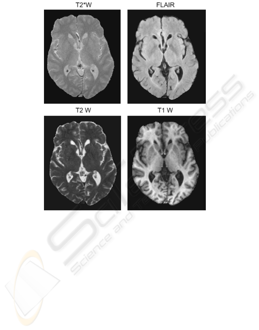
Figure 1: T2

∗

W, FLAIR, T2 W, T1 W, axial slice of coregistered sequences from a subject after brain extraction.

tral approach for segmenting tissue types in nor-

mal and abnormal brains, including white matter le-

sions (WMLs), based on mapping two magnetic res-

onance (MR) structural sequences in the red/green

colour space and using minimum variance quantisa-

tion (MVQ) to cluster and quantify the tissues. The

current study builds on that work.

For a relevant (albeit dated) comparison between a

supervised and an unsupervised clustering techniques

(neural networks) see (Hall et al., 1992). Due to

the advantages that unsupervised techniques have for

achieving an automatic segmentation process in re-

duced number of steps, we decided to evaluate the

performance of four well-known unsupervised clus-

tering algorithms k-means (MacQueen et al., 1966),

EM (Gaussian mixture) (Dempster et al., 1977),

MVQ (minimum variance quantization) (Xiang and

Joy, 1994) and Mean Shift (Comaniciu and Meer,

2002).

It is known that the use of two or more se-

quences increases the information at each voxel and

aids the automated classiﬁcation (Thacker and Jack-

son, 2001a). This paper addresses the problem of

fully automated detection of white matter/grey mat-

ter and CSF from a multisprectral image (we used T1

weighted, T2 weighted, T2

∗

weighted and FLAIR), in

an unsupervised setting.

The structure of the paper is as follows. Section

2 details the acquisition parameters of the scans in

question. Section 3 describes the actions performed

on the datasets before they were processed by the au-

tomated algorithms. Section 4 motivates the approach

and graphically explores the problem. Section (5) de-

scribes how the algorithms were validated and how

they operate. It addresses a subtle design choice re-

lating to whether the data should be analysed on a per

slice or volume basis. We then describe the cluster-

ing algorithms used, their merits and their disadvan-

tages. Section (6) states numerically how each algo-

rithm performed.

BIOSIGNALS 2010 - International Conference on Bio-inspired Systems and Signal Processing

508

2 MATERIALS

We use 12 sets of structural MR se-

quences from the Disconnected Mind Study

(http://www.disconnectedmind.org.uk), which

aims to understand how and why some older people’s

cognitive function deteriorates more than others,

and ﬁnd associations between brain physiology and

cognitive performance in a population of more than

1000 volunteers of the Lothian Birth Cohort 1936.

All MR images were rated for WML and atro-

phy using validated qualitative rating scales (Fazekas

et al., 2002; Longstreth et al., 1996; Wahlund et al.,

1990) by an experienced neuroradiologist (author

JMW). Based on these ratings, the sample for the

present work was selected so as to represent the full

range of WMLs across a range of degrees of brain at-

rophy. The MR sequences in this cohort study were:

• A T1-weighted (T1W) brain volume was ac-

quired (T R = 9ms; T E = 4ms; coronal acquisi-

tion). The 3D volume matrix size was 156×256×

256, with a voxel size of 1.3 × 1 ×1mm

• A T2-weighted (T2W) brain volume was ac-

quired (T R = 11300ms; T E = 100ms; axial ac-

quisition). The 3D volume matrix size was 80 ×

256 × 256, with a voxel size of 2 × 1 × 1mm

• A T2

∗

-weighted (T2

∗

W) brain volume was ac-

quired (T R = 940ms; T E = 15ms; axial acquisi-

tion). The 3D volume matrix size was 80×256 ×

256, with a voxel size of 2 × 1 × 1mm

• A FLAIR brain volume was acquired (T R =

9000ms; T E = 147ms; axial acquisition). The 3D

volume matrix size was 80 × 256 × 256, with a

voxel size of 2 × 1 × 1mm

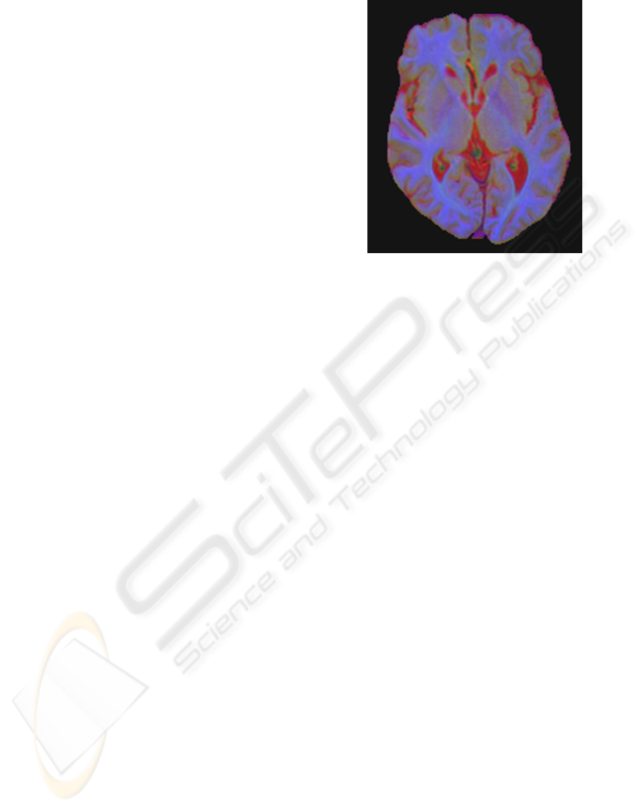
Figure 2 shows an axial slice of an individual’s

brain with 3 sequences (T2

∗

W, FLAIR and T1W)

fused into one image, with each one occupying a sin-

gle colour channel (red, green and blue, respectively).

Figure 1 shows the same slice, but as four separate

images. As described below, the images have been

rigidly co-registered and irrelevant material (such as

the skull) has been removed.

3 PREPROCESSING

Each set of four structural sequences per subject were

afﬁnely registered to each other using the FSL appli-

cation FLIRT (http://www.fmrib.ox.ac.uk/fsl/ﬂirt/).

FLIRT is an open source, command line linear reg-

istration tool maintained by the Analysis Group,

Figure 2: The T2

∗

W, FLAIR and T1W sequences fused in

red, green and blue channels, respectively.

FMRIB, Oxford, UK. The volumes were resam-

pled so that they were in the same space and con-

tain the same number of images. The intensities

were manually window-leveled in each volume so

that the intensity ranges in all images were approx-

imately the same. A mask of the brain was gen-

erated using the biomedical imaging software Ana-

lyze (http://www.analyzedirect.com), and in particu-

lar, its seeded region growing segmentation function-

ality, with stopping criteria dependant on thresholds.

The masks were checked for errors and any errors

were manually removed. The brain mask is used to

zero all intensities outside the brain.

4 INVESTIGATION/VALIDITY

A precondition for the previous work is that a given

voxel can be classiﬁed into one of the tissue types by

determining the intensities at that voxel together with

the intensity distribution across the entire image. A

ﬁrst step in determining the validity of this is to visu-

alise the intensity distributions for a given image.

In our context this distribution manifests itself as a

4D joint histogram or scatter plot as shown in Figure

It is evident that there are at least two obvious

clusters which may correspond to different tissue

types. Through experimentation these clusters have

been determined to be grey matter/white matter (i.e.

brain tissue) and CSF. In most projections the grey

matter/white matter cluster is small in extent but in

the T1W projections it has a large extent, with grey

matter at one end and white matter at the other end.

This highlights the fact that T1W is the best sequence

A COMPARISON OF FOUR UNSUPERVISED CLUSTERING ALGORITHMS FOR SEGMENTING BRAIN TISSUE

IN MULTI-SPECTRAL MR DATA

509

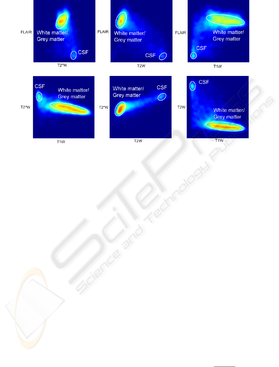
Figure 3: Joint histogram (or joint probability distribution) of the four sequences on a portion of the volume shown as

six 2D projections. Each view is an average projection and so represents the marginal probability density for the different

intensity types. The colour represents the probability/frequency at that point with dark blue representing low frequency and

red representing high frequency, on a log scale. The projections have been smoothed. Sequence values are increasing from

left to right and bottom to top. Contributions from the background (zero intensities) have been ignored and do not appear.

for segmenting grey from white matter because it pro-

vides the best contrast between them. It also high-

lights the fact that segmenting grey and white matter

from each other using intensity information only is

problematic because there is a continuum of intensity

ranges between them, with no obvious boundary.

The CSF cluster has high intensity on a T2W scan

and low intensity on T1W. The contrast between brain

tissue and CSF is high in T2W, which again is a

known result. In terms of volume, CSF represents a

far smaller proportion of the brain than brain tissue

and consequently this peak is not as pronounced as

the other.

The clear separation of CSF and brain tissue sug-

gests that an intensity based approach may work. Di-

rect thresholding at predeﬁned levels is unlikely to

work because of the natural variability in MR images

and because there may not be a threshold which sep-

arates them in any one sequence.

5 ALGORITHMIC

DETAILS/JUSTIFICATION

A precondition for the previous work is that a given

voxel can be classiﬁed by determining the intensi-

ties at that voxel together with the intensity distribu-

tion across the entire image. A fully automated clus-

tering algorithm analyses the intensity distributions

and partitions the intensity space into four clusters –

background, CSF, grey matter and white matter. The

boundaries between these clusters in feature space are

known as feature space decision boundaries.

5.1 Validation Details

The algorithms were evaluated numerically by com-

paring the automatically generated segmentations to

user collected segmentations which are considered to

be true (ground truth). We used standard comparison

metrics: true positive fraction (TPF), positive predic-

tive value (PPV) and Dice coefﬁcient. The TPF is the

fraction of ground truth which was found (in terms of

volume). The PPV is the fraction of the segmentation

which is correct (in terms of volume). The Dice coef-

ﬁcient combines these two measures into one. In all

cases a value of zero indicates a complete failure and

one indicates a complete success. To be speciﬁc, the

Dice metric is deﬁned as:

Dice(X,Y) =

2|X ∩Y |

|X| + |Y |

(1)

where X & Y are the ground truth and generated seg-

mentations, respectively.

BIOSIGNALS 2010 - International Conference on Bio-inspired Systems and Signal Processing

510

Presently, only the correctness of the CSF and

WM segmentations have been evaluated. Intuitively

CSF should be the easiest of the three tissue types to

segment because it seems to be well localised in the

joint histogram and well separated from the other tis-

sue types. On the other hand it might be the hardest

because it has a very high surface area to volume ratio

in comparison to the other tissue types. Since errors

are normally made at the boundary or surface of a re-

gion, those errors will represent a larger percentage

of the total volume of the tissue and so have a larger

effect on the Dice coefﬁcient.

The ground truth was provided by the SFC Brain

Imaging Research Centre. It was semi-automatically

generated using a method developed in-house in the

SFC Brain Imaging Research centre followed by

manual editing by an experienced image analyst (au-

thor MVH). This presents an obvious bias towards

the MVQ algorithm, and consequently the results pre-

sented with regard to the MVQ should be interpreted

with caution.

5.2 Per Slice/Per Volume Analysis

The question arrises as to whether the clustering pro-

cess should proceed on a per volume or per slice ba-

sis. That is, should the clustering algorithms draw

their samples from the entire volume or should they

perform the clustering on each slice individually?

One advantage of the per-slice strategy is a rel-

ative immunity to magnetic ﬁeld inhomogeneities at

least in the axial direction. Obviously the extent of

this advantage is tied to the severity of the magnetic

ﬁeld inhomogeneities, which in this experiment are

not signiﬁcant.

A disadvantage is that, although the total number

of samples in the feature space is the same in every

slice, 128×128, the number of samples in a given tis-

sue type is highly variable between slices. In slices

where a class does not appear in high frequency, there

is an increased risk that it will be incorrectly classi-

ﬁed.

Our investigation suggested that the per volume

strategy signiﬁcantly outperforms the other in both

total segmentation accuracy and consistency. Conse-

quently from this point on we will refer only to the

results of the whole volume analysis.

5.3 Clustering Algorithms

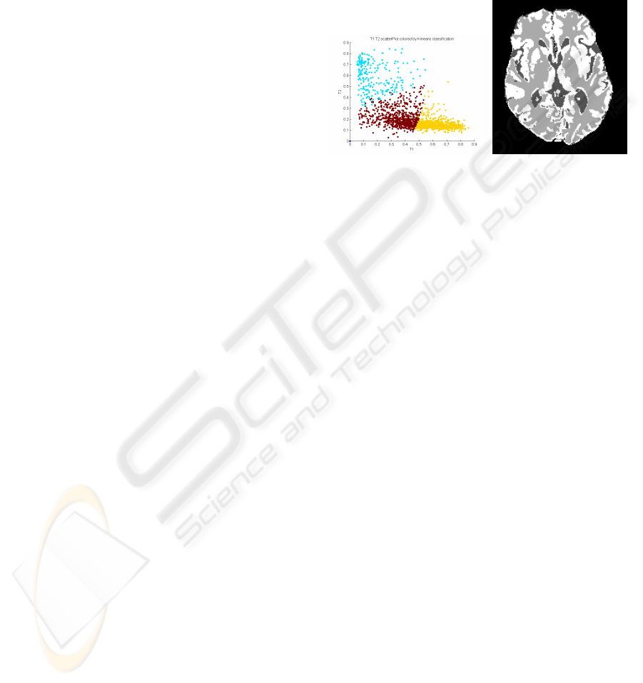
5.3.1 k-Means

The k-means algorithm is an iterative clustering al-

gorithm which, given a set of multidimensional data,

which it interprets as points in a Euclidean space, par-

titions it into a given number of clusters k such that

the sum of the Euclidean distance squared from each

point to its respective cluster center is approximately

minimal. The k-means algorithm (MacQueen et al.,

1966) can be applied directly to the intensities to ac-

quire a partition. In this experiment, four clusters are

Figure 4: k-means intensity classiﬁcations over T1W &

T2W. CSF, grey matter and white matter are coloured in

blue, red and yellow, respectively.

requested and the k-means search is initialised with

known approximate intensities for the different tis-

sue types. As expected, the feature space decision

boundaries on the resultant classiﬁer are composed

of straight hyper-planes in the 4-dimensional feature

space. It is almost certainly the case that the optimal

feature space decision boundaries, are not a collec-

tion of hyper-planes. Despite producing physically

unrealistic feature space decision boundaries in this

way, it has still performed well as shown in the results

section, and has chosen to split the white-matter/grey

matter distributions.

5.3.2 EM

The expectation-maximization (EM) algorithm ﬁnds

a set of statistical model parameters which best ex-

plains a given set of observed data, in the presence of

unobserved latent variables. It does this by determin-

ing the set of parameters which maximise the likeli-

hood of the data. The EM algorithm was explained

and given its name in (Dempster et al., 1977). It is an

iterative method that alternates between an expecta-

tion stage, which calculates the distribution of the la-

tent variables given the parameters of the model, and

a maximisation stage, which determines the set of pa-

rameters of the model that maximises the expectation

of the likelihood of the data. In the context of this

paper, we seek to model the joint probability density

function of the points within the brain as a function

of their intensities in each sequence. The probabilis-

tic model is deemed to be a mixture of a ﬁxed num-

ber of Gaussian distributions, where the means, co-

A COMPARISON OF FOUR UNSUPERVISED CLUSTERING ALGORITHMS FOR SEGMENTING BRAIN TISSUE

IN MULTI-SPECTRAL MR DATA

511

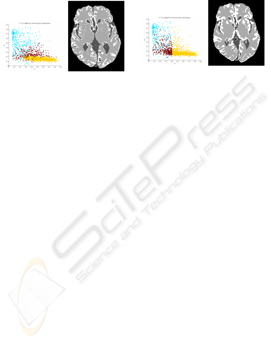
Figure 5: EM intensity classiﬁcations over T1W & T2W.

CSF, grey matter and white matter are coloured in blue, red

and yellow, respectively.

variances and weights of the Gaussians are allowed to

vary. In this case, the latent variables determine which

Gaussian distribution each sample belongs to. We ini-

tialise the EM algorithm with approximate parameters

which have been determined a priori to relate to tissue

types. Thus, once the EM algorithm has converged

and the Gaussian mixture has been determined, we

can directly assign a tissue type to each Gaussian dis-

tribution. We can then partition the image into tis-

sue types by determining which of the Gaussians it

is most likely a member of by using the maximum

posterior probably. For this experiment we removed

the background intensities from the set of voxels to

be classiﬁed because this caused the EM algorithm to

fail to converge. The minimum number of distribu-

tions for which the EM algorithm would give a sensi-

ble result was four. In practice, CSF was deemed to

be the union of two found class types, whereas grey

matter and white matter were represented by the other

2 classes.

The feature space decision boundaries produced

by this clustering algorithm can be shown to be com-

posed of quadratic surfaces, and so are, in general,

curved. This can be seen in ﬁgure 5. Intuitively, these

decision boundaries would be more like the optimal

decision boundaries by virtue of the fact that they are

curved. Despite this, it did not perform the best. In

general it seemed to over-segment the white matter

and under-segment grey matter. It also seemed to pro-

duce noisier segmentations.

5.3.3 MVQ

The minimum variance quantisation (MVQ) algo-

rithm (Xiang and Joy, 1994) is used in image process-

ing and compression for reducing the colour depth of

an image, for example, from 65535 to 256. It pro-

duces noticeably better quality images by respecting

the distributions of the colours in the image. More

speciﬁcally it aims to minimise the variance (sum

Figure 6: MVQ intensity classiﬁcations over T1W & T2W.

CSF, grey matter and white matter are coloured in blue, red

and yellow, respectively.

squared difference) between input image and the out-

put image. The class of partitions it considers are box

partitions (i.e. the partition surfaces are orthogonal

hyper-planes). In common with the other clustering

algorithms considered here, MVQ uses no spatial in-

formation. It can be interpreted as a clustering algo-

rithm and this is how it is used in this experiment. We

set the algorithm to quantise the number of colours

in the fused image to four, and these colours are in-

terpreted as the different tissue types. The algorithm

can be generalised to N dimensions but typically (as

in MATLAB’s implementation) it is limited to three

dimensions, (red, green, blue) and so we must ignore

one of the channels (T2W).

This algorithm performed very well, although pro-

duced some physically unrealistic feature space deci-

sion boundaries.

5.3.4 Mean Shift

The mean shift algorithm (Comaniciu and Meer,

2002) is a non-parametric feature space analysis tech-

nique, which determines the gradient in feature space

at any point. This can be used to ﬁnd basins of at-

traction which partition the space, and consequently

assign each point in the feature space to a cluster.

Unlike the other algorithms the user does not supply

the number of clusters as this is determined automati-

cally. Instead the user supplies a radial basis function

which is normally (as in this case) a spherically sym-

metric Gaussian distribution, centered at zero with a

speciﬁed variance (or scale). Increasing the variance

tends to decrease the number of clusters. For this ex-

periment the scale parameter was tuned until the num-

ber of clusters was three or four.

Despite being one of the more elegant of the

clustering algorithms, its slow runtime and inability

to discriminate white matter from grey matter con-

tributed to its early disqualiﬁcation, and so it has not

been quantitatively evaluated. Its slow runtime is ac-

credited to its MATLAB implementation (the others

BIOSIGNALS 2010 - International Conference on Bio-inspired Systems and Signal Processing

512

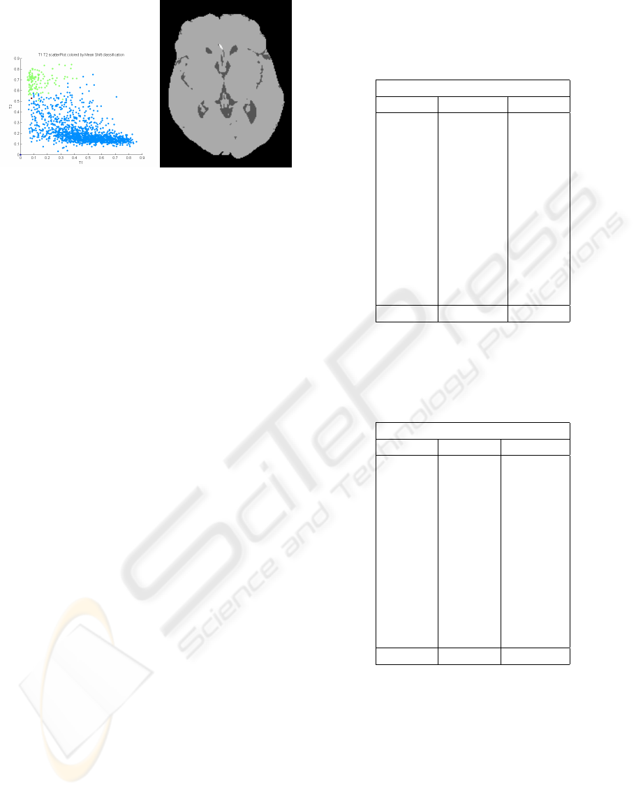
Figure 7: Mean shift intensity classiﬁcations over T1W &

T2W. CSF and grey matter/white matter are coloured in

green and blue, respectively.

are coded in C) and its inability to discriminate white

matter from grey matter is likely due to the fact that

they lie in the same attractive basin and so will never

be split into different partitions. On the other hand,

this clustering algorithm seemed to be very sensitive

to small but deﬁnite intensity features, and may prove

suited to the detection of pathologies such as WMLs

— this has not yet been investigated.

6 RESULTS AND DISCUSSION

The quantitative results from 12 datasets can be seen

in tables 1, 2 and 3. As explained above, the mean

shift algorithm has not been quantitatively evaluated.

Looking at the average Dice coefﬁcient for CSF we

see that MVQ performs best although the validation

is biased towards it (see section 5.1). EM also has

performed well, and has a number of desirable prop-

erties which the k-means or the MVQ lack, such as

the ability to assign a probability of a voxel being in

a given tissue classiﬁcation, which can improve vol-

ume measurement accuracy, see (Thacker and Jack-

son, 2001b), amongst other advantages. Looking at

the scores relating to white matter however, we see

that k-means performs best of all, with 91% accuracy.

ACKNOWLEDGEMENTS

These experiments were undertaken as part of an

EngD with ISLI (Institute of System Level Inte-

gration - http://www.isli.co.uk/ - EPSRC) as the

sponsor. The work was undertaken at SBIRC

(the SFC Scottish Imaging Research Centre -

http://www.sbirc.ed.ac.uk).

The datasets and ground truth used in these ex-

periments were collected as part of the Disconnected

Table 1: k-means: Dice coefﬁcients for CSF and white mat-

ter for the k-means clustering algorithm. Conﬁdence values

calculated at 99% using student-t distribution. White mat-

ter ground truth is missing for datasets Sub1, Sub2 and Sub3

and so these do not appear.

k-means

Dataset CSF WM

Sub1 .72

Sub2 .71

Sub3 .73

Z01 .72 .9

Z02 .72 .96

Z03 .73 .92

Z04 .81 .89

Z11 .73 .95

Z14 .74 .95

Z16 .78 .7

Z17 .77 .95

Z19 .7 .95

Average .74 ± .03 .91 ± .1

Table 2: MVQ: Dice coefﬁcients for CSF and white matter

for the MVQ clustering algorithm. Conﬁdence values cal-

culated at 99% using student-t distribution. White matter

ground truth is missing for datasets Sub1, Sub2 and Sub3

and so these do not appear.

MVQ

Dataset CSF WM

Sub1 .86

Sub2 .91

Sub3 .91

Z01 .91 .84

Z02 .92 .89

Z03 .87 .76

Z04 .91 .75

Z11 .91 .88

Z14 .9 .89

Z16 .85 .6

Z17 .92 .84

Z19 .9 .86

Average .9 ± .02 .81 ± .11

Mind Project (http://www.disconnectedmind.org.uk).

The Disconnected Mind Project is funded by Help

the Aged (http://www.helptheaged.org.uk/en-gb) and

the UK Medical Research Council. The SFC

Brain Imaging Centre is part of the Scottish Imag-

ing Network, a Platform for Scientiﬁc Excellence

(SINAPSE, http://www.sinapse.ac.uk); author JMW

is part funded by the SINAPSE collaboration.

Thanks to Ian Poole and Y. R. Petillot for their

involvement and input.

A COMPARISON OF FOUR UNSUPERVISED CLUSTERING ALGORITHMS FOR SEGMENTING BRAIN TISSUE

IN MULTI-SPECTRAL MR DATA

513

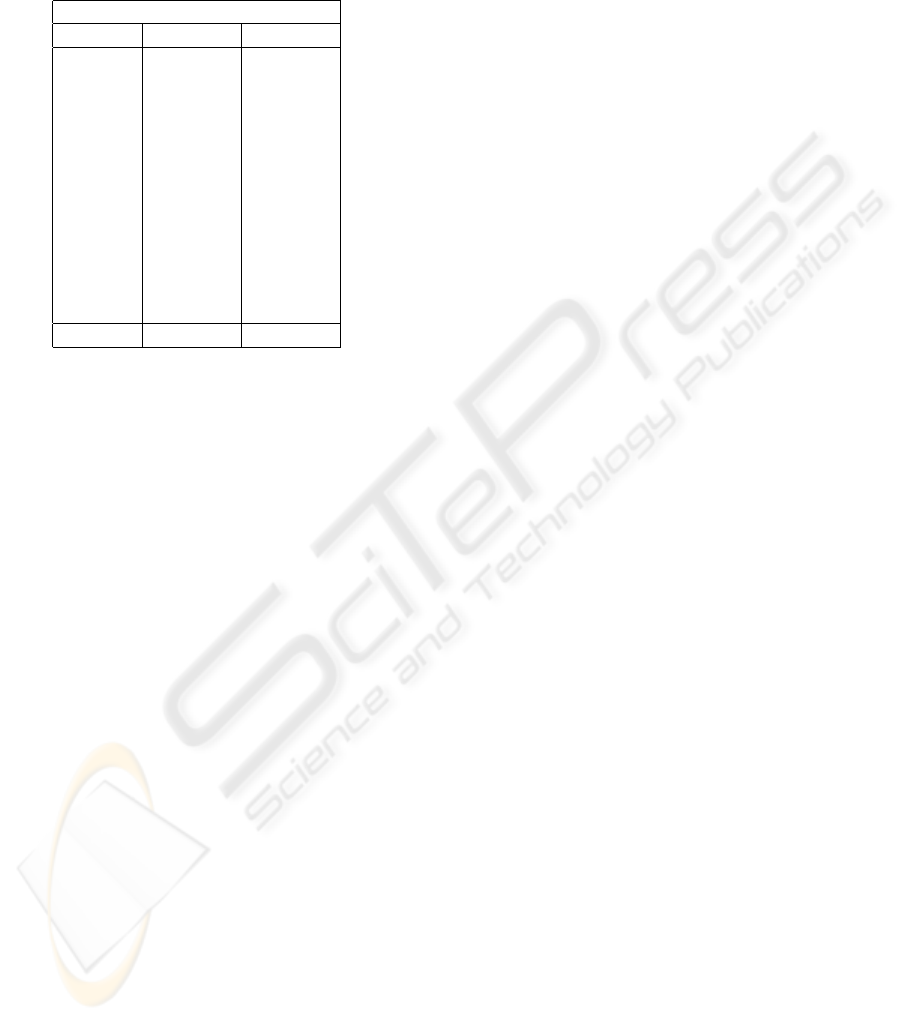
Table 3: EM: Dice coefﬁcients for CSF and white matter for

the EM clustering algorithm. Conﬁdence values calculated

at 99% using student-t distribution. White matter ground

truth is missing for datasets Sub1, Sub2 and Sub3 and so

these do not appear.

Dataset CSF WM

Sub1 .86

Sub2 .8

Sub3 .73

Z01 .7 .79

Z02 .68 .9

Z03 .75 .74

Z04 .76 .72

Z11 .83 .8

Z14 .78 .76

Z16 .81 .7

Z17 .76 .87

Z19 .71 .76

Average .76 ± .04 .78 ± .08

REFERENCES

Blatter, D., Bigler, E., Gale, S., Johnson, S., Anderson, C.,

Burnett, B., Parker, N., Kurth, S., and Horn, S. (1995).

Quantitative volumetric analysis of brain MR: norma-

tive database spanning 5 decades of life. American

Journal of Neuroradiology, 16(2):241–251.

Burton, E., Karas, G., Paling, S., Barber, R., Williams, E.,

Ballard, C., McKeith, I., Scheltens, P., Barkhof, F.,

and O’Brien, J. (2002). Patterns of cerebral atrophy in

dementia with Lewy bodies using voxel-based mor-

phometry. Neuroimage, 17(2):618–630.

Busatto, G., Garrido, G., Almeida, O., Castro, C., Camargo,

C., Cid, C., Buchpiguel, C., Furuie, S., and Bottino, C.

(2003). A voxel-based morphometry study of tempo-

ral lobe gray matter reductions in Alzheimers disease.

Neurobiology of aging, 24(2):221–231.

Comaniciu, D. and Meer, P. (2002). Mean shift: A robust

approach toward feature space analysis. IEEE Trans-

actions on pattern analysis and machine intelligence,

pages 603–619.

Crum, W. (2007). Spectral Clustering and Label Fusion For

3D Tissue Classiﬁcation: Sensitivity and Consistency

Analysis.

Dempster, A., Laird, N., Rubin, D., et al. (1977). Maxi-

mum likelihood from incomplete data via the EM al-

gorithm. Journal of the Royal Statistical Society. Se-

ries B (Methodological), 39(1):1–38.

Fazekas, F., Barkhof, F., Wahlund, L., Pantoni, L., Erkin-

juntti, T., Scheltens, P., and Schmidt, R. (2002). CT

and MRI rating of white matter lesions. Cerebrovas-

cular Diseases, 13:31–36.

Good, C., Johnsrude, I., Ashburner, J., Henson, R., Friston,

K., and Frackowiak, R. (2001). A voxel-based mor-

phometric study of ageing in 465 normal adult human

brains. Neuroimage, 14(1):21–36.

Hall, L., Bensaid, A., Clarke, L., Velthuizen, R., Silbiger,

M., and Bezdek, J. (1992). A comparison of neural

network and fuzzy clustering techniques insegment-

ing magnetic resonance images of the brain. IEEE

Transactions on Neural Networks, 3(5):672–682.

Head, D., Snyder, A., Girton, L., Morris, J., and Buckner,

R. (2005). Frontal-hippocampal double dissociation

between normal aging and Alzheimer’s disease. Cere-

bral Cortex, 15(6):732–739.

Lehtovirta, M., Laakso, M., Soininen, H., Helisalmi, S.,

Mannermaa, A., Helkala, E., Partanen, K., Ryyn

anen,

M., Vainio, P., Hartikainen, P., et al. (1995). Vol-

umes of hippocampus, amygdala and frontal lobe in

Alzheimer patients with different apolipoprotein E

genotypes. Neuroscience, 67(1):65–72.

Longstreth, W., Manolio, T., Arnold, A., Burke, G., Bryan,

N., Jungreis, C., Enright, P., O’Leary, D., and Fried,

L. (1996). Clinical correlates of white matter ﬁndings

on cranial magnetic resonance imaging of 3301 el-

derly people The Cardiovascular Health Study. Stroke,

27(8):1274–1282.

MacQueen, J. et al. (1966). Some methods for classiﬁcation

and analysis of multivariate observations.

Miller, A., Alston, R., and Corsellis, J. (1980). Variation

with age in the volumes of grey and white matter in

the cerebral hemispheres of man: measurements with

an image analyser. Neuropathology and applied neu-

robiology, 6(2):119–132.

Murgasovaa, M. (2009). Construction of a dynamic 4D

probabilistic atlas for the developing brain.

Pham, D., Xu, C., and Prince, J. (2000). Current Methods

In Medical Image Segmentation 1. Annual Review of

Biomedical Engineering, 2(1):315–337.

Thacker, N. and Jackson, A. (2001a). Mathematical seg-

mentation of grey matter, white matter and cerebral

spinal ﬂuid from MR image pairs. British Journal of

Radiology, 74(879):234.

Thacker, N. and Jackson, A. (2001b). Mathematical seg-

mentation of grey matter, white matter and cerebral

spinal ﬂuid from MR image pairs. British Journal of

Radiology, 74(879):234.

Vrooman, H., Cocosco, C., van der Lijn, F., Stokking, R.,

Ikram, M., Vernooij, M., Breteler, M., and Niessen,

W. (2007). Multi-spectral brain tissue segmentation

using automatically trained k-nearest-neighbor classi-

ﬁcation. Neuroimage, 37(1):71–81.

Wahlund, L., Agartz, I., Almqvist, O., Basun, H., Forssell,

L., Saaf, J., and Wetterberg, L. (1990). The brain in

healthy aged individuals: MR imaging. Radiology,

174(3):675–679.

Xiang, Z. and Joy, G. (1994). Color image quantization by

agglomerative clustering. IEEE Computer Graphics

and Applications, 14(3):44–48.

BIOSIGNALS 2010 - International Conference on Bio-inspired Systems and Signal Processing

514