
NORMAL SYNTHESIS ON RGBN IMAGES
Thiago Pereira and Luiz Velho
Vision and Graphics Laboratory, Instituto de Matematica Pura e Aplicada, Brazil
Keywords:
RGBN, Texture synthesis, Normal map, Filtering.
Abstract:
In this work, we synthesize normals and color to add geometric details to an RGBN image (image with a
color and a normal channel). Existing modeling and image processing tools are not apt to edit RGBN images
directly. Since high resolution RGBN images can be obtained using photometric stereo, we used them as full
models and as exemplars in a Texture from Example synthesis.
Our method works on RGBN images by combining the normals from two bands: base shape and details. We
use a high pass filter to extract a texture exemplar, which is synthesized over the model’s smooth normals,
taking into account foreshortening corrections. We also discuss conditions on the exemplars and models that
guarantee that the resulting normal image is a realizable surface.
1 INTRODUCTION
We use texture synthesis to edit large regions of an
RGBN image changing both color and normals. The
RGBN image (Toler-Franklin et al., 2007) is a 2.5D
data type since it is a photo containing, for each pixel,
not only color but also geometry information (nor-
mal). Editing regions by individually addressing local
changes can be painstaking to artists. For this reason
this process needs to be made automatic. Two options
arise. Procedural methods are very powerful but are
in general difficult to control. We use a texture from
example method that takes as input only a small sam-
ple of the desired texture and then reproduces it in a
large region. Our system can synthesize normal tex-
tures on shapes represented by normals (RGBN im-
ages), never using positions. Regarding synthesis, an
advantage of working with RGBN images is that the
projective mapping distortions on the synthesized tex-
tures can be corrected by using information from the
normals. The texture sticks to the surface.
However, we do not want the texture to follow
every small surface irregularity. Therefore, we sep-
arate the RGBN image into macro and mesostructure
bands. It is common to cluster different geometric
scales in different levels (Chen et al., 2006). The
macrostructure level is the general shape of the model
as would be seen from a distance. The mesostructure
level contains intermediate geometric details that are
visible with a naked eye such as bumps and creases.
Our synthesis method can respect the base shape, only
changing the details.
Our method can be applied to RGBN images from
many different sources. A high-resolution modeled
mesh can be used to extract it and enhance models
with fewer polygons (Cohen et al., 1998; Cignoni
et al., 1998). Further processing of details of this
model can proceed using the normal map and avoid-
ing a huge mesh. An alternative to modelling is cap-
turing real-world objects. Capturing normals with 3D
scanning requires expensive equipment and lacks res-
olution, being far behind the cheaper digital cameras.
Better results come from photometric approaches as
in the digitization of Michelangelo’s Pieta (Bernardini
et al., 2002). A projective atlas (Velho and Sossai Jr.,
2007) can be built from this dataset. The resulting
charts are surfaces mapped by a camera transforma-
tion to the image plane. Since they contain normal
and colors, each chart is in fact an RGBN and can be
edited by our system.
Capturing a model’s normals is easy using photo-
metric stereo techniques (Woodham, 1989). It takes
as input multiple images from the same view point,
each illuminated with different known light positions.
It then solves a least-squares problem to find the nor-
mal and albedo (color) of each pixel in the image.
Since photometric stereo works on regular images,
it allows the capture of very high resolution models.
This is a powerful method to obtain full models but
also to generate texture exemplars.
Our main contributions are:
1. Synthesizing normal vectors allowing relighting
13
Pereira T. and Velho L. (2010).
NORMAL SYNTHESIS ON RGBN IMAGES.
In Proceedings of the International Conference on Computer Graphics Theory and Applications, pages 13-20
DOI: 10.5220/0002813800130020
Copyright
c
SciTePress
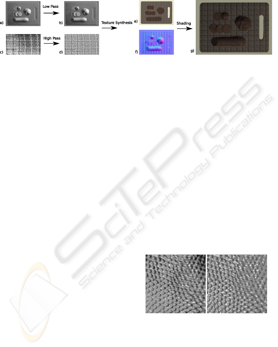
Figure 1: Overview of the method. Inputs: a) RGBN image, c) texture exemplar. Filtered inputs: b) smooth RGBN image, d)
texture detail. Results: e) color, f) normal (represented in RGB colors) and g) shaded RGBN image.
of the final model.
2. An RGBN image editing system implementing a
frequency aware texture synthesis framework sep-
arating exemplars and models into base shape and
details.
In section 3, we present an overview of our nor-
mal synthesis framework. In section 4, we discuss
the work of (Zelinka et al., 2005) in color synthesis on
RGBN images. In section 5, we extend their method
for synthesizing normals. In section 6, we determine
when the edited RGBN images correspond to a real-
izable surface.
2 RELATED WORK
Texture from example synthesis can be classified into
two approaches. In pixel-based methods, new pix-
els are generated one at a time. In (Efros and Leung,
1999), the authors search for a best match between
the neighborhood of the already synthesized texture
and neighborhoods in the texture sample. There are
also patch-based methods (Efros and Freeman, 2001)
(Fang and Hart, 2004) where the algorithm step con-
sists of iteratively synthesizing small regions at a
time. This approach leads to a direct transfer of local
statistics, but it has the drawback that seams between
patches need to be handled.
Another classification of synthesis regards the do-
main. Texture synthesis can be parametric, volume-
based or manifold-based. Volume-based methods will
synthesize texture usually in R
2
or R
3
. Parametric
synthesis will target more general manifolds by work-
ing in the parametric domain (usually planar). There
are also manifold methods which are non-parametric
(Wei and Levoy, 2001) (Turk, 2001). These methods
work directly in the manifold representation (usually
a mesh) and use only local decisions.
In (Zelinka et al., 2005; Fang and Hart, 2004)
the authors extend manifold techniques to work on
RGBN images, using the normal as a local descrip-
tor of shape. Both works use shape from shading
to recover normals from photographs. Normals are
used to guide distortions in the synthesized color tex-
ture. Zelinka (Zelinka et al., 2005) adapted jump map
based synthesis which is a pixel based method to work
on normals, while Textureshop(Fang and Hart, 2004)
uses a patch based method. Both works allow for ad-
vanced editing of images. For example, object mate-
rial can be replaced, while still respecting shape and
shading. Unlike these works, in our method, both
color and normals are synthesized on RGBN images.
One way of looking at RGBN synthesis is as a quasi-
stationary process (Zhang et al., 2003). Synthesis pro-
ceeds through the image but varies spatially depend-
ing on the normals.
In (Haro et al., 2001), the authors capture high res-
olution normals of small patches of face skin and then
use texture synthesis to replicate these tangent space
normals in parametric space. Adding detail to faces
is an important application of our method. While
in their approach, a normal map is synthesized from
scratch, we can respect existing frequency bands in
the normal map. Procedural synthesis was explored
in (Kautz et al., 2001) where bump maps are created
on the fly based on a normal density function.
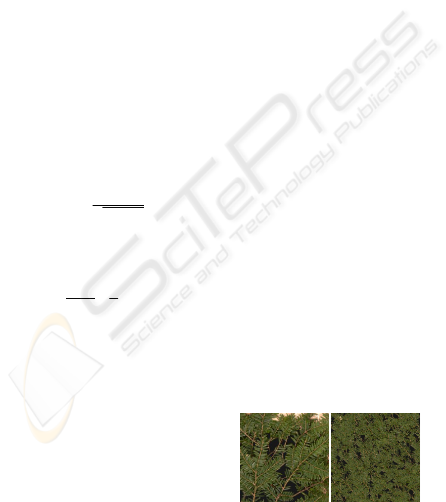
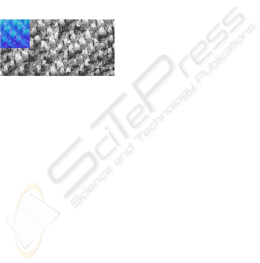
(a) Original Exemplar (b) Filtered Exemplar
Figure 2: Removing the normal low frequencies of the ex-
emplar only the desired details. We show shaded images of
the normals under same lighting conditions.
GRAPP 2010 - International Conference on Computer Graphics Theory and Applications
14
3 METHOD
While the problem of synthesizing color textures on
top of RGBN models has been studied in (Zelinka
et al., 2005), we propose a method to synthesize nor-
mal textures. We start this section with an overview
of our method (Figure 1). The method receives as
input an RGBN image (a) and an RGBN examplar
(c). It has three steps. First, in the frequency split-
ting step, we low-pass filter the normal image (b) re-
moving details and we high-pass filter the examplar
normals (d) removing the base shape. Second, in the
texture synthesis step, we synthesize both the colors
(e) and normals (f) of the examplar on the smooth nor-
mals (b) compensating for foreshortening distortions.
Finally, in the combination step, we merge the synthe-
sized normal details with the smooth RGBN image.
To build the smooth normals we use the RGBN
bilateral filter (Toler-Franklin et al., 2007). It takes
into account both normal and color differences and
respects edges. In (Pereira and Velho, 2009), the au-
thors have developed linear filters for normals that al-
lows any kernel mask to be used. It builds on the one
to one mapping between a normal field N(x, y) and the
gradient field (z
x
, z
y
) of an associated height function
z given by:
N(x,y) =
(−z
x
, −z
y
, 1)
q
z
2
x
+ z
2
y
+ 1
To filter normals, they first convert it to a height
gradient. By noting that derivatives and convolution
(g kernel) commute, the gradients can be filtered as if
we had the height function z at hand.
(z ∗g)
x
=
∂(z ∗g)
∂x
=
∂z
∂x
∗ g = (z
x
∗ g)
During splitting, we use their high pass kernel on
the texture sample (Figure 2). As an alternative to
the bilateral filter we could build the smooth normals
using a low pass kernel. The filters in (Pereira and
Velho, 2009) have the advantage that they guarantee
that the resulting normals correspond to a surface.
To assist the user in defining the editing region, we
use a segmentation method (Felzenszwalb and Hut-
tenlocher, 2004) which was extended (Toler-Franklin
et al., 2007) to handle RGBN images. The procedure
is fast and is well suited to interactive applications. It
also takes into account the normal and color channels,
using all available information to improve results. It
is also possible to segment objects based solely on
geometry. To avoid over-segmenting, a bilateral filter
should be used prior to segmentation to remove noise
while preserving edges.
For replicating the RGBN sample on a base
RGBN, we extended jump map-based texture syn-
thesis (Zelinka and Garland, 2004), more specifi-
cally jump maps on RGBN images (Zelinka et al.,
2005). This method is non-parametric and pixel-
based, avoiding the need of a local parametrizations
on normal maps. It does not produce the best qual-
ity results but it is the only interactive time technique,
allowing for easy user experimentation. This strategy
also handles base geometry distortions by varying im-
age edge lengths during synthesis as a function of the
normals.
During texture synthesis, colors are defined for
each pixel. However the synthesized normals (high
frequency) still have to be combined with the filtered
input normals (low frequencies). We want to com-
bine normals controlling which frequency bands we
are replacing or editing. We follow the approach of
(Pereira and Velho, 2009), where two combination
schemes were proposed: the linear model and the ro-
tation model. The linear model combines normals by
looking at them as gradients. This strategy is sim-
pler and has the advantage that the resulting normals
are guaranteed to correspond to a real surface, but the
equivalent position displacements are restricted to the
z-direction. On the other hand, the rotation model de-
forms the details to follow the base shape before com-
bining. We use this method for all examples.
4 JUMPMAPS ON RGBNS
We begin this section by reviewing jump map-based
texture synthesis on a regular image. We also describe
a few principles that makes the method better suited to
our application. We then discuss (Zelinka et al., 2005)
the extension to color synthesis on RGBN images.
The simple example-based synthesis algorithms
(Efros and Leung, 1999; Efros and Freeman, 2001)
exhaustively search the input for a best match. This
search is done for each pixel or patch being synthe-
sized. In (Zelinka and Garland, 2004), Zelinka splits
texture synthesis in two phases: analysis and syn-
thesis. Note that in previous methods analysis was
Figure 3: Jump Map synthesis results.
NORMAL SYNTHESIS ON RGBN IMAGES
15
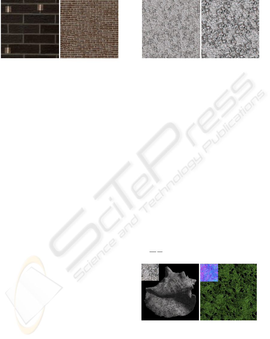
Figure 4: The highlighted neighborhoods are similar, but a
jump between them introduces offsets, breaking brick align-
ment. A bigger mask size (19x19) improves results.
being done online and would use an already synthe-
sized neighborhood as a query. Zelinka’s insight is
that while this neighborhood is only known at synthe-
sis time it will resemble an existing one in the tex-
ture example. As such, we can precalculate and store
the similarities between all neighborhoods in the ex-
amplar. The Jump Map data structure holds for each
examplar pixel a list of jumps to similar pixels.
During synthesis, the output texture is traversed
and pixels are sequentially copied from the example.
Eventually the input texture border will be reached,
that is when the jump map comes in hand. As the
border approaches, a jump is randomly selected from
the Jump Map. As such, there is an infinite amount of
texture to be copied.
The analysis phase is cast as a nearest-neighbor
(NN) problem in a neighborhood space. Each pixel’s
square neighborhood is encoded in an M
2
feature vec-
tor, using the L
2
norm for comparisons. Notice that
two parameters influence performance M and N (in-
put sample size). Since analysis with small values of
M won’t represent the texture appropriately we are
easily led to a high dimensional NN problem which
would be too slow to handle directly. Instead, the au-
thors use an approximate nearest neighbors (ANN)
data structure (Mount, 1998) that allows very fast
queries. For further optimization, PCA is used for
dimensionality reduction of the feature vector.
As Zelinka notices, jump map synthesis works
best for stochastic textures and weak structured tex-
tures. While quality results can be obtained with
highly structured textures (Figure 10), these are ex-
ceptions. The reason can be seen in Figure 4. We
see very similar neighborhoods, but if a jump is taken
between them offsets will be introduced in the synthe-
sized bricks. This problem happened because a small
neighborhood was used for analysis. While increas-
ing M improves results, it also increases analysis time.
For highly structured textures it is more important
to match structure than to transfer details. We use
multiresolution to ignore sample details during analy-
Figure 5: In both images, analysis was done with a 100x100
sample, but the second was synthesized with a 500x500
higher resolution sample, which would be hard to analyze.
sis. We notice that it is possible to use different values
of N (different resolutions) for analysis and synthesis,
virtually allowing larger masks. We use small sam-
ples for fast analysis, while we use detailed samples
for quality synthesis (Figure 5). Zelinka uses mul-
tiresolution but only to improve PCA compression.
To extend this algorithms to RGBN images, two
problems have to be solved: synthesizing normals
and synthesizing on normal images. The next sec-
tion presents our solution to the first problem. To
handle the second one (Zelinka et al., 2005) adapted
jump map-based color synthesis to normal images.
On RGBN images, we need to vary the scale of the
synthesis spatially due to foreshortening (Figure 6-
a). A unit pixel offset in the output image induces
a displacement in the represented surface, which in
turns induces an offset in texture space. These param-
eters may be global or may vary smoothly over the
surface (Zhang et al., 2003). By approximating the
surface locally by a plane orthogonal to the normal
n, we can obtain the displacement d
t
in texture space
as a function of the displacement d
i
in output image
space and of the projection p of d
i
onto the surface
d
t
=
|d
i
|
|n
z
|
p
|p|
, p = d
i
− < n, d
i
> n.
(a) (b)
Figure 6: a) Due to foreshortening, texture scale varies spa-
tially according to the normals. b) The leaves were repli-
cated generating a normal map. We show here a shaded
version of the synthesized map.
GRAPP 2010 - International Conference on Computer Graphics Theory and Applications
16
5 NORMAL TEXTURES
We have extended the analysis and synthesis steps
of the jump maps method to synthesize normals. In
the analysis phase, we take a normal map sample
representing our desired texture and we are asked
to build a jump map for it. Since the basic prim-
itive in jump map analysis is comparing neighbor-
hoods, we must settle on which metric to use. In
the color setting, the sum of the euclidean metric for
each pixel neighborhood was used. However normals
are in the unit-sphere S
2
and as a consequence each
neighborhood feature vector is in the cartesian prod-
uct S
2
× S
2
× ... × S
2
. Therefore, the sum of the pixel
normal metrics will induce a natural definition of a
neighborhood metric, we only have to choose a nor-
mal metric. We analyze three different metrics: eu-
clidean, geodesic and dot product based.
The geodesic distance obtained from the angle
cos
−1
(< n
1
, n
2
>) is a natural choice (intrinsic dis-
tance) and it would be easy to adapt the O(N
2
) so-
lution to the NN problem in the analysis phase. On
the other hand, since cos
−1
is a non-linear function, it
is very hard to adapt either PCA or ANN, the funda-
mental algorithms that allow building jump maps in
reasonable time. Linearity could be obtained by us-
ing a dot product based distance 1− < n
1
, n
2
>, but
it falls far from the geodesic distance (Figure 7) spe-
cially for small values. In NN problems, these are the
exactly the ones we are most interested in. This leads
us to our last metric alternative: Euclidean. The Eu-
clidean metric is a very good approximation for the
geodesic metric for small distances since their deriva-
tives at zero agree. Therefore, the Euclidean distance
gives us a good compromise between simplicity and
precision, so this is our choice for texture analysis.
As for synthesis, the order in which pixels of the
output image are synthesized is important to reduce
directionality bias. This happens because each pixel
is synthesized based on only one of its neighbors.
Zelinka found that following Hilbert curves produces
much better results than scan-line or serpentine traver-
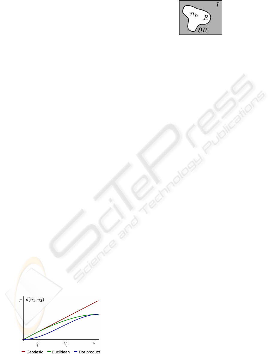
Figure 7: Different normal distances as function of the an-
gle between the normals.
Figure 8: The detail normals n
h
defined in R are combined
with the image normals.
sals. However, we do not use Hilbert traversal. The
reason is we look for synthesis in subsets of RGBN
images, which could be defined by either user or au-
tomated segmentation. Since these regions may have
very complex shapes and topologies, it would be com-
plicated to use a synthesis order based on Hilbert
curves. Instead, we used a depth-first search (DFS)
using a 4-connected pixel neighborhood. We recur-
sively visit each pixels and its neighbors. The naive
DFS algorithm produces unpleasant results with a di-
rectionality bias. This is a consequence of always
visiting a fixed neighbor first, for example the north
neighbor. A simple alternative is to use DFS, proceed-
ing to each cardinal direction in random order. This
breaks directionality and generates results almost as
good as Hilbert traversal ones, as demonstrated by all
results in this manuscript. The DFS traversal has two
advantages. First, it only processes the pixels being
synthesized. Second, it can respect discontinuities in
the normals. For instance, in Figure 6-a we would
not want synthesis to cross from the upper part of the
shell to the lower part, we would like them to be in
different connected components in the graph. This is
easy to handle, if two neighboring pixels have differ-
ent normals (defined by a threshold), they are simply
not connected in the graph.
6 INTEGRABILITY ANALYSIS
In this section, we discuss the conditions for the re-
sulting normals to be integrable, that is, for it to cor-
respond to a surface. For simplicity, we only analyze
the linear combination method (Section 3) and disre-
gard the foresight distortions introduced by scaling.
Given a base normal field n
b
defined in the entire
image I (Figure 8) and a synthesized detail normal
field n
h
defined in R ⊂ I, the problem of combining
normals is generating a new normal field which agrees
with n
b
everywhere, but is influenced in R by n
h
. We
refer to their respective height functions as b and h.
We can look at a normal image n as a 2D vector
field w (Section 3). If this field is the gradient of
a height function, we say it is a conservative vector
field. This means our normal image does correspond
NORMAL SYNTHESIS ON RGBN IMAGES
17
to a surface.
The authors of (Pereira and Velho, 2009) show
that conservative results can be guaranteed when
combining normals by adding their vector fields coun-
terparts w
h
and w
b
. Three conditions must be satis-
fied. First of all, they require w
h
and w
b
to be con-
servative. Second, since h is only defined in R, we
must extend it as zero outside the edited region. This
requires w
h
to fall smoothly to zero close to ∂R and
be equal to 0 outside. However this is not enough the
added detail must not introduce level changes outside
R or it will create discontinuities in height.
Figure 9: When the low frequencies of the exemplar are
not removed, it is harder to infer pattern. This generates an
uneven result.
What restrictions do we have to make to guarantee
that normal synthesis satisfies the three requirements
above? To begin with, w
h
might not fall smoothly or
not even fall to zero in ∂R, which would result in dis-
continuities in w. In many applications (Figure 10),
w
b
is already discontinuous in ∂R so that new discon-
tinuities are not created. Second, synthesis will not
introduce level changes if w
h
only contains high fre-
quency content which tends to oscillate and cancel it-
self. Hence, the restriction on w
h
is enforced with
the high-pass filter on the exemplars. In addition, tex-
ture synthesis methods in general, and jump maps in
particular, do not introduce repetitions and so no low
frequencies are created.
It seems very unlikely that non-parametric tex-
ture synthesis methods can guarantee the generation
of conservative fields in arbitrary domains, since only
local operations are performed. On the other hand,
local operations seem enough to generate curl-free
fields that guarantee that w is conservative under the
additional hypothesis that R is simply connected (does
not contain holes). Traditional techniques aim at gen-
erating texture such that each pixel’s neighborhood
closely resembles a neighborhood in the exemplar.
We argue that the curl is also similar in this neighbor-
hood. This means given curl-free exemplars, the syn-
thesis will generate approximately curl-free textures.
As Figure 10 shows, quality results can be obtained
even when R is not simply connected.
7 RESULTS
In this section, we will discuss some of the results ob-
tained. Shaded images were produced with one light
source. In some examples, uniform albedo is used
to better highlight shape. In Figure 12-b, only the
normals of the shell were changed, colors were unaf-
fected. The base geometry was combined with high
frequency normals extracted from rust. These new
normals retain the original shape of the shell but give
the appearance of a new material. It is true that with
some trial and error rust could be generated with a
procedural noise. On the other hand, structures syn-
thesis from real objects on the shell (Figure 12-c, 13)
can only be accomplished with texture from example
methods. These structured examples show how syn-
thesized details follow the base geometry.
In Figure 6-b, we can see a normal map sampled
from scanned leaves and synthesized normals. Uni-
form albedo was used for shading. There are some
aliasing artifacts which could be handled by synthe-
sizing in a higher resolution and down-sampling. This
is possible, since synthesis time scales linearly.
The original model contained a wooden board
with real vegetables (see Figure 10, upper left). Seg-
mentation was able to separate the objects. We added
the relief and color of the armor of a stone Chinese
warrior to the board. The complex topology of this
object was not a problem and DFS was able to guide
synthesis around it. Rust was synthesized on the veg-
etables (normal and color). The fine scale normals on
the normal map are hard to spot on the shaded version.
In Figure 9, a sample of the normals of a pine
cone was used for synthesis. Low frequencies were
not removed. This can be seen as the exemplar varies
smoothly from light (top) to dark blue (bottom). It
has two consequences, first it is harder for the analy-
sis phase to infer pattern. Second the final result is un-
even. The shaded image shows some darker regions
which are not facing the light.
As in Textureshop (Fang and Hart, 2004), shape
from shading can be used to recover normals from
photographs. We have also used it to obtain the tex-
ture exemplar (Figure 11). A swatch was extracted
from the lizard’s arm (b) and combined with smooth
hand normals (d). The final image (e) was shaded
under diffuse lighting, ignoring the lizard’s skin re-
flectance properties. For more realistic results, a syn-
thesis method that can handle morphing between tex-
tures is required. Notice how the texture of the fin-
gers, the hand and the arm of the lizard are differ-
ent. Very high frequency detail like human hand lines
could be recombined in the final result.
GRAPP 2010 - International Conference on Computer Graphics Theory and Applications
18
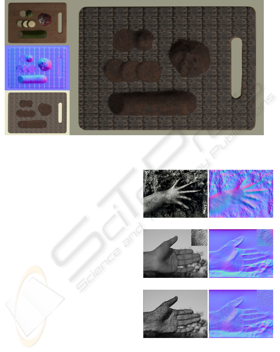
Figure 10: A shaded image of edited vegetables. Automatic segmentation followed by texture synthesis is a powerful tool for
material replacement. The vegetables were turned into rust metal.
8 CONCLUSIONS
We have developed a method to synthesize normal
textures on RGBNs. Our pipeline includes normal fil-
tering to control which frequency bands we edit or
replace. We discuss conditions on the exemplars and
models that guarantee that the resulting normal image
is a realizable surface.
Requiring the deformations to extend to 0 out-
side R is a limitation of our method, blending tech-
niques should be investigated in the future to en-
force this property on any synthesized deformation.
A limitation of jump map-based synthesis is that be-
ing pixel-based, it has problems with very structured
textures. On the other hand, it is harder to adapt
less local methods to RGBN images, since the met-
ric of bigger neighborhoods is non-trivial. In future
work, we would like to use normal synthesis in the
context of inpainting normals to fill missing regions.
Another direction is to use a projective atlas (Velho
and Sossai Jr., 2007) to extend this work to a surface.
This new synthesis would take into account not only
macrostructure (mesh) but also mesostructure in the
form of existing normal maps.
(a) Texture source (b) Normal map
(c) Original color (d) Original normals
(e) Shaded image (f) Synthesized normals
Figure 11: Shape from shading was used to estimate nor-
mals (b,d). A small sample of the lizard’s arm was filtered
and synthesized over the hand (e). Lighting (e) was set sim-
ilar to the original. Only the normals were used to produce
the final result.
NORMAL SYNTHESIS ON RGBN IMAGES
19
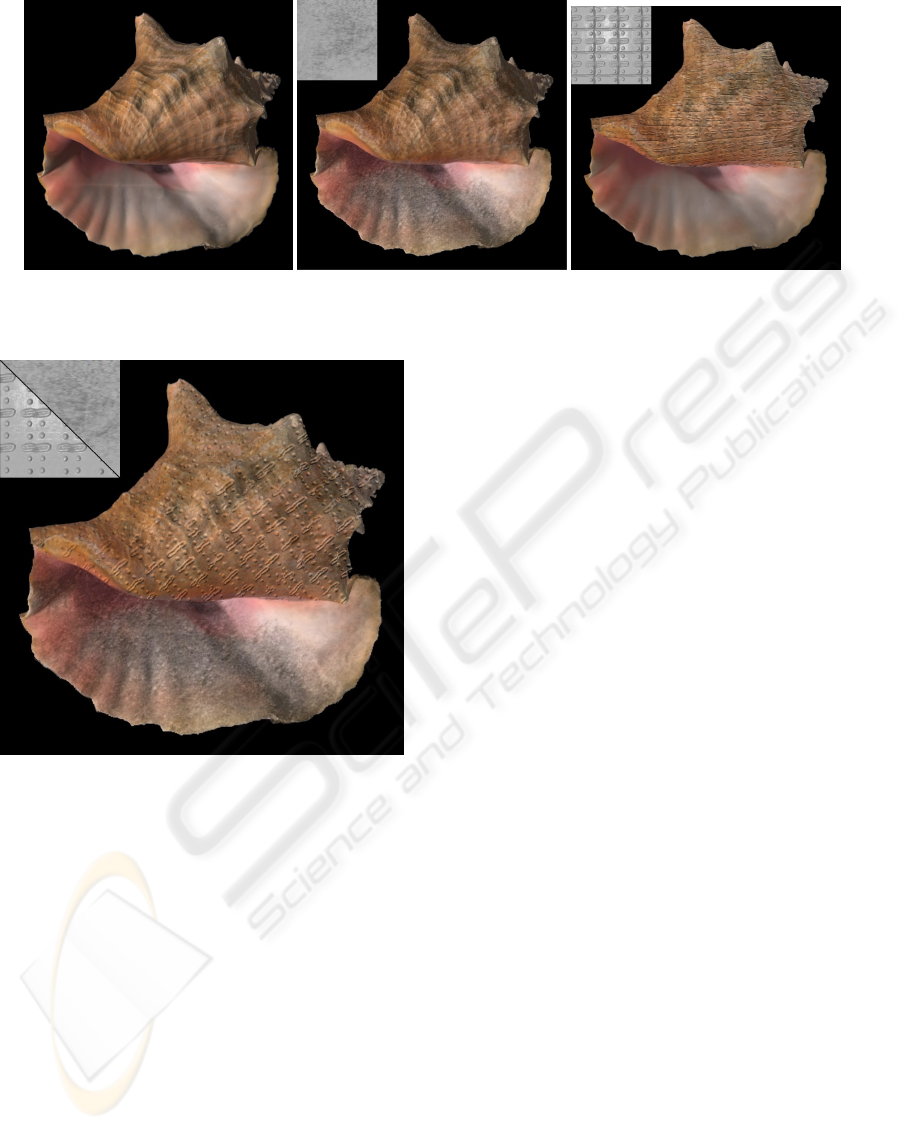
(a) Original Shell (b) Rust Normals (c) Armor Normals
Figure 12: The small images show the exemplars used under a direct light source. Images are embedded in high resolution.
Figure 13: Structured texture synthesis.
REFERENCES
Bernardini, F., Rushmeier, H., Martin, I. M., Mittleman,
J., and Taubin, G. (2002). Building a digital model
of michelangelo’s florentine pieta. IEEE Computer
Graphics and Applications.
Chen, T., Goesele, M., and Seidel, H.-P. (2006). Mesostruc-
ture from specularity. In IEEE CVPR ’06.
Cignoni, P., Montani, C., Scopigno, R., and Rocchini, C.
(1998). A general method for preserving attribute val-
ues on simplified meshes. In VIS ’98: Proceedings of
the conference on Visualization ’98. IEEE Computer
Society Press.
Cohen, J., Olano, M., and Manocha, D. (1998).
Appearance-preserving simplification. In SIGGRAPH
’98. ACM.
Efros, A. and Leung, T. (1999). Texture synthesis by non-
parametric sampling. In ICCV ’99. IEEE Computer
Society.
Efros, A. A. and Freeman, W. T. (2001). Image quilting
for texture synthesis and transfer. In SIGGRAPH ’01.
ACM.
Fang, H. and Hart, J. C. (2004). Textureshop: texture syn-
thesis as a photograph editing tool. In SIGGRAPH
’04. ACM.
Felzenszwalb, P. F. and Huttenlocher, D. P. (2004). Efficient
graph-based image segmentation. Int. J. Comput. Vi-
sion, 59(2):167–181.
Haro, A., Essa, I. A., and Guenter, B. K. (2001). Real-
time photo-realistic physically based rendering of fine
scale human skin structure. Proceedings of the 12th
Eurographics Workshop on Rendering Techniques.
Kautz, J., Heidrich, W., and Seidel, H.-P. (2001). Real-time
bump map synthesis. HWWS ’01: EUROGRAPHICS
workshop on Graphics hardware.
Mount, D. M. (1998). Ann programming manual. Technical
report.
Pereira, T. and Velho, L. (2009). Rgbn image editing. Pro-
ceedings of SIBGRAPI.
Toler-Franklin, C., Finkelstein, A., and Rusinkiewicz, S.
(2007). Illustration of complex real-world objects us-
ing images with normals. In NPAR.
Turk, G. (2001). Texture synthesis on surfaces. In SIG-
GRAPH ’01. ACM.
Velho, L. and Sossai Jr., J. (2007). Projective texture at-
las construction for 3d photography. Vis. Comput.,
23(9):621–629.
Wei, L.-Y. and Levoy, M. (2001). Texture synthesis over
arbitrary manifold surfaces. In SIGGRAPH ’01. ACM.
Woodham, R. J. (1989). Photometric method for determin-
ing surface orientation from multiple images. pages
513–531.
Zelinka, S., Fang, H., Garland, M., and Hart, J. C. (2005).
Interactive material replacement in photographs. In
GI ’05: Proceedings of Graphics Interface 2005.
Zelinka, S. and Garland, M. (2004). Jump map-based
interactive texture synthesis. ACM Trans. Graph.,
23(4):930–962.
Zhang, J., Zhou, K., Velho, L., Guo, B., and Shum, H.-Y.
(2003). Synthesis of progressively-variant textures on
arbitrary surfaces. In SIGGRAPH ’03. ACM.
GRAPP 2010 - International Conference on Computer Graphics Theory and Applications
20
