HYPERACCURATE ELLIPSE FITTING WITHOUT ITERATIONS
Kenichi Kanatani
Department of Computer Science, Okayama University, Okayama 700-8530, Japan
Prasanna Rangarajan
Department of Electrical Engineering, Southern Methodist University, Dallas, TX 75205, U.S.A.
Keywords:
Ellipse fitting, Least squares, Algebraic fit, Error analysis, Bias removal.
Abstract:
This paper presents a new method for fitting an ellipse to a point sequence extracted from images. It is widely
known that the best fit is obtained by maximum likelihood. However, it requires iterations, which may not
converge in the presence of large noise. Our approach is algebraic distance minimization; no iterations are
required. Exploiting the fact that the solution depends on the way the scale is normalized, we analyze the
accuracy to high order error terms with the scale normalization weight unspecified and determine it so that the
bias is zero up to the second order. We demonstrate by experiments that our method is superior to the Taubin
method, also algebraic and known to be highly accurate.
1 INTRODUCTION
Circular objects are projected onto camera images as
ellipses, and from their 2-D shapes one can recon-
struct their 3-D structure (Kanatani, 1993). For this
reason, detecting ellipses in images and computing
their mathematical representation are the first step of
many computer vision applications including indus-
trial robotic operations and autonomous navigation.
This is done in two stages, although they are often in-
termingled. The first stage is to detect edges, test if a
particular edge segment can be regarded as an elliptic
arc, and integrate multiple arcs into ellipses (Kanatani
and Ohta, 2004; Rosin Rosin and West, 1995). The
second stage is to fit an equation to those edge points
regarded as constituting an elliptic arc. In this paper,
we concentrate on the latter.
Among many ellipse fitting algorithms presented
in the past, those regarded as the most accurate are
methods based on maximum likelihood (ML), and
various computational schemes have been proposed
including the FNS (Fundamental Numerical Scheme
of Chojnacki et al. (2000), the HEIV (Heteroscedas-
tic Errors-in-Variable of Leedan and Meer (2000) and
Matei and Meer (2006), and the projective Gauss-
Newton iterations of Kanatani and Sugaya (2007).
Efforts have also been made to make the cost func-
tion more precise (Kanatani and Sugaya, 2008) and
add a posterior correction to the solution (Kanatani,
2006), but the solution of all ML-based methods al-
ready achieves the theoretical accuracy limit, called
the KCR lower bound (Chernov and Lesort, 2004;
Kanatani, 1996; Kanatani, 2008), up to high order er-
ror terms. Hence, there is practically no room for fur-
ther accuracy improvement. However, all ML-based
methods have one drawback: Iterations are required
for nonlinear optimization, but they often fail to con-
verge in the presence of large noise. Also, an appro-
priate initial guess must be provided. Therefore, ac-
curate algebraic methods that do not require iterations
are very much desired, even though the solution may
not be strictly optimal.
The best known algebraic method is the least
squares, also known as algebraic distance minimiza-
tion or DLT (direct linear transformation) (Hartley
and Zisserman, 2004), but all algebraic fitting meth-
ods have an inherent weakness: We need to impose
a normalization to remove scale indeterminacy, yet
the solution depends on the choice of the normaliza-
tion. Al-Sharadqah and Chernov (2009) and Rangara-
jan and Kanatani (2009) exploited this freedom for fit-
ting circles. Invoking the high order error analysis of
Kanatani (Kanatani, 2008), they optimized the nor-
malization so that the solution has the highest accu-
racy. In this paper, we apply their techniques to ellipse
fitting. Doing numerical experiments, we demon-
5
Kanatani K. and Rangarajan P. (2010).
HYPERACCURATE ELLIPSE FITTING WITHOUT ITERATIONS.
In Proceedings of the International Conference on Computer Vision Theory and Applications, pages 5-12
DOI: 10.5220/0002814500050012
Copyright
c
 SciTePress

strate that our method is superior to the method of
Taubin (1991), also an algebraic method known to be
very accurate (Kanatani, 2008; Kanatani and Sugaya,
2007).
2 ALGEBRAIC FITTING
An ellipse is represented by
Ax
2
+ 2Bxy+Cy
2
+ 2f
0
(Dx+ Ey) + f
2
0
F = 0, (1)
where f
0
is a scale constant that has an order of x and
y; without this, finite precision numerical computa-
tion would incur serious accuracy loss
1
. Our task is
to compute the coefficients A, ..., F so that the ellipse
of Eq. (1) passes through given points (x
α
,y
α
), α = 1,
..., N, as closely as possible. The algebraic approach
is to compute A, ..., F that minimize the algebraic dis-
tance
J=
1
N
N
∑
α=1

Ax
2
α
+ 2Bx
α
y
α
+Cy
2
α
+ 2f
0
(Dx
α
+ Ey
α
)
+ f
2
0
F

2
. (2)
This is also known as the least squares, algebraic dis-
tance minimization, or the direct linear transforma-
tion (DLT). Evidently, Eq. (2) is minimized by A =
··· = F = 0 if no scale nomalization is imposed. Fre-
quently used normalizations include
F = 1, (3)
A+ D = 1, (4)
A
2
+ B
2
+C
2
+ D
2
+ E
2
+ F
2
= 1, (5)
A
2
+ B
2
+C
2
+ D
2
+ E
2
= 1, (6)
A
2
+ 2B
2
+C
2
= 1, (7)
AC − B
2
= 1. (8)
Equtation (3) reduces minimization of Eq. (2) to si-
multatneous linear equations (Albano, 1974; Cooper
and Yalabik, 1976, Rosin, 1993). However, Eq. (1)
with F = 1 cannot represent ellipses passing through
the origin (0,0). Equation (4) remedies this (Gander
et al., 1994; Rosin, 1994). The most frequently used
is
2
Eq. (5) (Paton, 1970), but some authors use Eq. (6)
(Gnanadesikan, 1977). Equation (7) imposes invari-
ace to coordiate transformations in the sense that the
ellipse fitted after the coordinate system is transalated
1
In our experiments, we set f
0
= 600, assuming images
of one side less than 1000 pixels.
2
Some authors write an ellipse as Ax
2
+ Bxy + Cy
2
+
Dx + Ey + F = 0. The meaning of Eq. (5) differs for this
form and for Eq. (1). In the following, we ignore such small
differences; no significant consequence would result.
and rotated is the same as the originally fitted ellipse
translated and rotated afterwards (Bookstein, 1979).
Equation (8) prevents Eq. (1) from representing a
parabola (AC− B
2
= 0) or a hyperbola (AC− B
2
< 0)
(Fitzgibbon et al., 1999). Many other normalizations
are conceivable, but the crucial fact is that the result-
ing solution depends on which normalization is im-
posed. The purpose of this paper is to find the “best”
normalization. Write the 6-D vector of the unknown
coefficients as
θ =

A B C D E F

⊤
, (9)
and consider the class of normalizations written as
(θ,Nθ) = constant, (10)
for some symmetric matrix N, where and hereafter we
denote the inner product of vectors a an b by (a, b).
Equations (5), (6), and (7) can be written in this form
with a positive definite or semidefinite N, while for
Eq. (8) N is nondefinite. In this paper, we allow non-
definite N, so that the constant in Eq. (10) is not nec-
essarily positive.
3 ALGEBRAIC SOLUTION
If the weight matrix N is given, the solution θ that
minimizes Eq. (1) is immediately computed. Write
ξ =

x
2
2xy y
2
2f
0
x 2f
0
y f
2
0

⊤
. (11)
Equation (1) is now written as
(θ,ξ) = 0. (12)
Let ξ
α
be the value of ξ for (x
α
,y
α
). Our problem is
to minimize
J =
1
N
N
∑
α=1
(θ,ξ
α
)
2
=
1
N
N
∑
α=1
θ
⊤
ξ
α
ξ
⊤
α
θ = (θ,Mθ),
(13)
subject to Eq. (10), where we define the 6× 6 matrix
M as follows:
M =
1
N
N
∑
α=1
ξ
α
ξ
⊤
α
. (14)
Equation (13) is a quadratic form in θ, so it is mini-
mized subject to Eq. (10) by solving the generalized
eigenvalue problem
Mθ = λNθ. (15)
If Eq. (1) is exactly satisfied for all (x
α
,y
α
), i.e.,
(θ,ξ
α
) = 0 for all α, Eq. (14) implies Mθ = 0 and
hence λ = 0. If the weight N is positive definite or
semidefinite, the generalized eigenvalue λ is positive
VISAPP 2010 - International Conference on Computer Vision Theory and Applications
6

in the presence of noise, so the solution is given by the
generalized eigenvectorθ for the smallest λ. Here, we
allow N to be nondefinite, so λ may not be positive.
In the following, we do error analysis of Eq. (15) by
assuming that λ ≈ 0, so the solution is given by the
generalized eigenvector θ for the λ with the small-
est absolute value
3
. Since the solution θ of Eq. (15)
has scale indeterminacy, we hereafter adopt normal-
ization into unit norm kθk = 1 rather than Eq. (10).
The resulting solution may not necessarily repre-
sent an ellipse; it may represent a parabola or hy-
perbola. This can be avoided by imposing Eq. (8)
(Fitzgibbon et al., 1999), but here we do not exclude
nonellipse solution and optimize N so that the result-
ing solution θ is as close to its true value θ as possible.
Least Squares. In the following, we call the popu-
lar method of using Eq. (5) the least squares for
short. This is equivalent to letting N to be the unit
matrix I. In this case, Eq. (15) becomes an ordi-
nary eigenvalue problem
Mθ = λθ, (16)
and the solution is the unit eigenvector of M for
the smallest eigenvalue.
Taubin Method. A well known algebraic method
known to be very accurate is due to Taubin (1991),
who used as N
N
T
=
4
N
N
∑
α=1








x
2
α
x
α
y
α
0 f
0
x
α
0 0
x
α
y
α
x
2
α
+ y
2
α
x
α
y
α
f
0
y
α
f
0
x
α
0
0 x
α
y
α
y
2
α
0 f
0
y
α
0
f
0
x
α
f
0
y
α
0 f
2
0
0 0
0 f
0
x
α
f
0
y
α
0 f
2
0
0
0 0 0 0 0 0








.
(17)
The solution is given by the unit generalized
eigenvector θ of Eq. (15) for the smallest gener-
alized eigenvalue λ.
4 ERROR ANALYSIS
We regard each (x
α
,y
α
) as perturbed from its true po-
sition ( ¯x
α
, ¯y
α
) by (∆x
α
,∆y
α
) and write
ξ
α
=
¯
ξ
α
+ ∆
1
ξ
α
+ ∆
2
ξ
α
, (18)
where
¯
ξ
α
is the true value of ξ
α
, and ∆
1
ξ
α
, and ∆
2
ξ
α
are the noise terms of the first and the second order,
respectively:
3
In the presence of noise, M is positive definite, so
(θ,Mθ) > 0. If (θ, Nθ) < 0 for the final solution, we have
λ < 0. However, if we replace N by −N, we obtain the
same solution θ with λ > 0, so the sign of λ does not have
a particular meaning.
∆
1
ξ
α
=







2¯x
α
∆x
α
2¯x
α
∆y
α
+2¯y
α
∆x
α
2¯y
α
∆y
α
2f
0
∆x
α
2f
0
∆y
α
0







, ∆
2
ξ
α
=







∆x
2
α
2∆x
α
∆y
α
∆y
2
α
0
0
0







.
(19)
The second term ∆
2
ξ
α
is ellipse specific and was not
considered in the general theory of Kanatani (2008).
We define the covariance matrix of ξ
α
by V[ξ
α
] =
E[∆
1
ξ
α
∆
1
ξ
⊤
α
], where E[·] denotes expectation. If the
noise terms ∆x
α
and ∆y
α
are regarded as independent
random Gaussian variables of mean 0 and standard
deviation σ, we obtain
V[ξ
α
] = E[∆
1
ξ
α
∆
1
ξ
⊤
α
] = σ
2
V
0
[ξ
α
], (20)
where we put
V
0
[ξ
α
] = 4








¯x
2
α
¯x
α
¯y
α
0 f
0
¯x
α
0 0
¯x
α
¯y
α
¯x
2
α
+ ¯y
2
α
¯x
α
¯y
α
f
0
¯y
α
f
0
¯x
α
0
0 ¯x
α
¯y
α
¯y
2
α
0 f
0
¯y
α
0
f
0
¯x
α
f
0
¯y
α
0 f
2
0
0 0
0 f
0
¯x
α
f
0
¯y
α
0 f
2
0
0
0 0 0 0 0 0








. (21)
Here, we have noted that E[∆x
α
] = E[∆y
α
] = 0, E[∆x
2
α
]
= E[∆y
2
α
] = σ
2
, and E[∆x
α
∆y
α
] = 0 according to our
assumption. We call the above V
0
[ξ
α
] the normalized
covariance matrix. Comparing Eqs. (21) and (17), we
find that the Taubin method uses as N
N
T
=
1
N
N
∑
α=1
V
0
[ξ
α
], (22)
after the observations (x
α
,y
α
) are plugged into
( ¯x
α
, ¯y
α
).
5 PERTURBATION ANALYSIS
Substituting Eq. (18) into Eq. (14), we have
M=
1
N
N
∑
α=1
(
¯
ξ
α
+ ∆
1
ξ
α
+ ∆
2
ξ
α
)(
¯
ξ
α
+ ∆
1
ξ
α
+ ∆
2
ξ
α
)
⊤
=
¯
M+ ∆
1
M+ ∆
2
M+ ··· , (23)
where ··· denotes noise terms of order three and
higher, and we define
¯
M, ∆
1
M, and ∆
2
M by
¯
M =
1
N
N
∑
α=1
¯
ξ
α
¯
ξ
⊤
α
, (24)
∆
1
M =
1
N
N
∑
α=1

¯
ξ
α
∆
1
ξ
⊤
α
+ ∆
1
ξ
α
¯
ξ
⊤
α

, (25)
HYPERACCURATE ELLIPSE FITTING WITHOUT ITERATIONS
7

∆
2
M =
1
N
N
∑
α=1

¯
ξ
α
∆
2
ξ
⊤
α
+ ∆
1
ξ
α
∆
1
ξ
⊤
α
+ ∆
2
ξ
α
¯
ξ
⊤
α

.
(26)
We expand the solution θ and λ of Eq. (16) in the form
θ =
¯
θ+ ∆
1
θ+ ∆
2
θ+ ··· , λ =
¯
λ+ ∆
1
λ+ ∆
2
λ+ ··· ,
(27)
where the barred terms are the noise-free values, and
symbols ∆
1
and ∆
2
indicate the first and the second
order noise terms, respectively. Substituting Eqs. (23)
and (27) into Eq. (15), we obtain
(
¯
M+ ∆
1
M+ ∆
2
M+ ···)(
¯
θ+ ∆
1
θ+ ∆
2
θ+ ···)
=(
¯
λ+∆
1
λ+∆
2
λ+···)N(
¯
θ+∆
1
θ+∆
2
θ+···). (28)
Expanding both sides and equating terms of the same
order, we obtain
¯
M
¯
θ =
¯
λN
¯
θ, (29)
¯
M∆
1
θ+ ∆
1
M
¯
θ =
¯
λN∆
1
θ+ ∆
1
λN
¯
θ, (30)
¯
M∆
2
θ+ ∆
1
M∆
1
θ+ ∆
2
M
¯
θ
=
¯
λN∆
2
θ+ ∆
1
λN∆
1
θ+ ∆
2
λN
¯
θ. (31)
The noise-free values
¯
ξ
α
and
¯
θ satisfy (
¯
ξ
α
,
¯
θ) = 0, so
Eq. (24) implies
¯
M
¯
θ = 0, and Eq. (29) implies
¯
λ = 0.
From Eq. (25), we have (
¯
θ,∆
1
M
¯
θ) = 0. Computing
the inner product of
¯
θ and Eq. (30), we find that ∆
1
λ
= 0. Multiplying Eq. (30) by the pseudoinverse
¯
M
−
from left, we have
∆
1
θ = −
¯
M
−
∆
1
M
¯
θ, (32)
where we have noted that
¯
θ is the null vector of
¯
M
(i.e.,
¯
M
¯
θ = 0) and hence
¯
M
−
¯
M (≡ P
¯
θ
) represents
orthogonal projection along
¯
θ. We have also noted
that equating the first order terms in the expansion of
k
¯
θ + ∆
1
θ + ∆
2
θ + ··· k
2
= 1 results in (
¯
θ,∆
1
θ) = 0so
P
¯
θ
∆
1
θ = ∆
1
θ. Substituting Eq. (32) into Eq. (31), we
can express ∆
2
λ in the form
∆
2
λ =
(
¯
θ,∆
2
M
¯
θ) − (
¯
θ,∆
1
M
¯
M
−
∆
1
M
¯
θ)
(
¯
θ,N
¯
θ)
=
(
¯
θ,T
¯
θ)
(
¯
θ,N
¯
θ)
,
(33)
where
T = ∆
2
M− ∆
1
M
¯
M
−
∆
1
M. (34)
Next, we consider the second order error ∆
2
θ.
Since
¯
θ is a unit vector and does not change its norm,
we are interested in the error component orthogonal
to
¯
θ. We define the orthogonal component of ∆
2
θ by
∆
⊥
2
θ = P
¯
θ
∆
2
θ (=
¯
M
−
¯
M∆
2
θ). (35)
Multiplying Eq. (31) by
¯
M
−
from left and substituting
Eq. (32), we obtain
∆
⊥
2
θ= ∆
2
λ
¯
M
−
N
¯
θ+
¯
M
−
∆
1
M
¯
M
−
∆
1
M
¯
θ −
¯
M
−
∆
2
M
¯
θ
=
(
¯
θ,T
¯
θ)
(
¯
θ,N
¯
θ)
¯
M
−
N
¯
θ−
¯
M
−
T
¯
θ. (36)
6 COVARIANCE AND BIAS
6.1 General Algebraic Fitting
From Eq. (32), we see that the leading term of the
covariance matrix of the solution θ is given by
V[θ] = E[∆
1
θ∆
1
θ
⊤
] =
¯
M
−
E[(∆
1
Mθ)(∆
1
Mθ)
⊤
]
¯
M
−
=
1
N
2
¯
M
−
E
h
N
∑
α=1
(∆ξ
α
,θ)
¯
ξ
α
N
∑
β=1
(∆ξ
β
,θ)
¯
ξ
⊤
β
i
¯
M
−
=
1
N
2
¯
M
−
N
∑
α,β=1
(θ,E[∆ξ
α
∆ξ
⊤
β
]θ)
¯
ξ
α
¯
ξ
⊤
β
¯
M
−
=
σ
2
N
2
¯
M
−

N
∑
α=1
(θ,V
0
[ξ
α
]θ)
¯
ξ
α
¯
ξ
⊤
α

¯
M
−
=
σ
2
N
¯
M
−
¯
M
′
¯
M
−
, (37)
where we define
¯
M
′
=
1
N
N
∑
α=1
(
¯
θ,V
0
[ξ
α
]θ)
¯
ξ
α
¯
ξ
⊤
α
. (38)
In the derivation of Eq. (37), we have noted that ξ
α
is
independent for different α and that E[∆
1
ξ
α
∆
1
ξ
⊤
β
] =
δ
αβ
σ
2
V
0
[ξ
α
], where δ
αβ
is the Kronecker delta. The
important observation is that the covarinace matrix
V[θ] of the solution θ does not depend on the nor-
malization weight N. This implies that all algebraic
methods have the same the covariance matrix in the
leading order, so we are unable to reduce the covari-
ance of θ by adjusting N. Yet, the Taubin method is
known to be far accurate than the least squares. We
will show that this stems from the bias terms and that
a superior method can result by reducing the bias.
Since E[∆
1
θ] = 0, there is no bias in the first order:
the leading bias is in the second order. In order to
evaluate the second order bias E[∆
⊥
2
θ], we evaluate
the expectation of T in Eq. (34). We first consider the
term E[∆
2
M]. From Eq. (26), we see that
E[∆
2
M]=
1
N
N
∑
α=1

¯
ξ
α
E[∆
2
ξ
α
]
⊤
+ E[∆
1
ξ
α
∆
1
ξ
⊤
α
]
+E[∆
2
ξ
α
]
¯
ξ
⊤
α

=
σ
2
N
N
∑
α=1

¯
ξ
α
e
⊤
13
+V
0
[ξ
α
] + e
13
¯
ξ
⊤
α

=σ
2

N
T
+ 2S [
¯
ξ
c
e
⊤
13
]

, (39)
where we have noted the definition in Eq. (20) and
used Eq. (22). The symbol S [·] denotes symmetriza-
tion (S [A] ≡ (A+ A
⊤
)/2), and the vectors
¯
ξ
c
and e
13
are defined by
VISAPP 2010 - International Conference on Computer Vision Theory and Applications
8

¯
ξ
c
=
1
N
N
∑
α=1
¯
ξ
α
, e
13
=

101000

⊤
. (40)
We nextconsider the term E[∆
1
M
¯
M
−
∆
1
M]. It has the
form (see Appendix for the derivation)
E[∆
1
M
¯
M
−
∆
1
M] =
σ
2
N
2
N
∑
α=1

tr[
¯
M
−
V
0
[ξ
α
]]
¯
ξ
α
¯
ξ
⊤
α
+(
¯
ξ
α
,
¯
M
−
¯
ξ
α
)V
0
[ξ
α
] + 2S [V
0
[ξ
α
]
¯
M
−
¯
ξ
α
¯
ξ
⊤
α
]

, (41)
where tr[·] denotes the trace. From Eqs. (39) and (41),
the matrix T in Eq. (34) has the followingexpectation:
E[T] = σ
2

N
T
+ 2S [
¯
ξ
c
e
⊤
13
]
−
1
N
2
N
∑
α=1

tr[
¯
M
−
V
0
[ξ
α
]]
¯
ξ
α
¯
ξ
⊤
α
+ (
¯
ξ
α
,
¯
M
−
¯
ξ
α
)V
0
[ξ
α
]
+2S [V
0
[ξ
α
]
¯
M
−
¯
ξ
α
¯
ξ
⊤
α
]

. (42)
Thus, the second order error ∆
⊥
2
θ in Eq. (36) has the
following bias:
E[∆
⊥
2
θ] =
¯
M
−

(
¯
θ,E[T]
¯
θ)
(
¯
θ,N
¯
θ)
N
¯
θ− E[T]
¯
θ

. (43)
6.2 Least Squares
Eq. (42) implies (
¯
ξ
c
,
¯
θ) = 0 and (
¯
ξ
α
,
¯
θ) = 0. Hence,
E[T]
¯
θ can be written as
E[T]
¯
θ = σ
2

N
T
¯
θ+ (A+C)
¯
ξ
c
−
1
N
2
N
∑
α=1

(
¯
ξ
α
,
¯
M
−
¯
ξ
α
)V
0
[ξ
α
]
¯
θ+(
¯
θ,V
0
[ξ
α
]
¯
M
−
¯
ξ
α
)
¯
ξ
α

.
(44)
If we let N = I, we obtain the least squares fit. Its
leading bias is
E[∆
⊥
2
θ] =
¯
M
−

(
¯
θ,E[T]
¯
θ)
¯
θ− E[T]
¯
θ

=−
¯
M
−
(I−
¯
θ
¯
θ
⊤
)E[T]
¯
θ = −
¯
M
−
E[T]
¯
θ, (45)
where we have used the following equality:
¯
M
−
(I−
¯
θ
¯
θ
⊤
) =
¯
M
−
P
¯
θ
=
¯
M
−
¯
M
¯
M
−
=
¯
M
−
. (46)
From Eqs. (44), and (45), the leading bias of the least
square has the following form:
E[∆
⊥
2
θ] = −σ
2
¯
M
−

N
T
¯
θ+ (A+C)
¯
ξ
c
−
1
N
2
N
∑
α=1

(
¯
ξ
α
,
¯
M
−
¯
ξ
α
)V
0
[ξ
α
]
¯
θ+(
¯
θ,V
0
[ξ
α
]
¯
M
−
¯
ξ
α
)
¯
ξ
α

.
(47)
6.3 Taubin Method
Eq. (44) implies (
¯
ξ
c
,
¯
θ) = 0 and (
¯
ξ
α
,
¯
θ) = 0. Hence,
(
¯
θ,E[T]
¯
θ) can be written as
(
¯
θ,E[T]
¯
θ)
=σ
2

(
¯
θ,N
T
¯
θ) −
1
N
2
N
∑
α=1
(
¯
ξ
α
,
¯
M
−
¯
ξ
α
)(
¯
θ,V
0
[ξ
α
]
¯
θ)

=σ
2

(
¯
θ,N
T
¯
θ) −
1
N
2
N
∑
α=1
tr[
¯
M
−
¯
ξ
α
¯
ξ
⊤
α
](
¯
θ,V
0
[ξ
α
]
¯
θ)

=σ
2

(
¯
θ,N
T
¯
θ) −
1
N
2
tr[
¯
M
−
N
∑
α=1
(
¯
θ,V
0
[ξ
α
]
¯
θ)
¯
ξ
α
¯
ξ
⊤
α
]

=σ
2
(
¯
θ,N
T
¯
θ) −
σ
2
N
tr[
¯
M
−
¯
M
′
], (48)
where we have used Eq. (38). If we let N = N
T
, we
obtain the Taubin method. Thus, the leading bias of
the Taubin fit has form
E[∆
⊥
2
θ] = −σ
2
¯
M
−

qN
T
¯
θ+ (A+C)
¯
ξ
c
−
1
N
2
N
∑
α=1

(
¯
ξ
α
,
¯
M
−
¯
ξ
α
)V
0
[ξ
α
]
¯
θ+(
¯
θ,V
0
[ξ
α
]
¯
M
−
¯
ξ
α
)
¯
ξ
α

,
(49)
where we put
q =
1
N
tr[
¯
M
−
¯
M
′
]
(
¯
θ,N
T
¯
θ)
. (50)
Comparing Eqs. (49) and (47), we notice that the only
difference is that N
T
¯
θ in Eq. (47) is replaced by qN
T
¯
θ
in Eq. (49). We see from Eq. (50) that q < 1 when N
is large. This can be regarded as one of the reasons
of the high accuracy of the Taubin method, as already
pointed out by Kanatani (2008).
6.4 Hyperaccurate Algebraic Fit
Now, we present our main contribution of this paper.
Our proposal is to chose the weight N to be
N = N
T
+ 2S [
¯
ξ
c
e
⊤
13
] −
1
N
2
N
∑
α=1

tr[
¯
M
−
V
0
[ξ
α
]]
¯
ξ
α
¯
ξ
⊤
α
+(
¯
ξ
α
,
¯
M
−
¯
ξ
α
)V
0
[ξ
α
] + 2S [V
0
[ξ
α
]
¯
M
−
¯
ξ
α
¯
ξ
⊤
α
]

. (51)
Then, we have E[T] = σ
2
N from Eq. (42), and
Eq. (43) becomes
E[∆
⊥
2
θ] = σ
2
¯
M
−

(
¯
θ,N
¯
θ)
(
¯
θ,N
¯
θ)
N− N

¯
θ = 0. (52)
Since Eq. (51) contains the true values
¯
ξ
α
and
¯
M, we
evaluate them by replacing the true values ( ¯x
α
, ¯y
α
) in
HYPERACCURATE ELLIPSE FITTING WITHOUT ITERATIONS
9

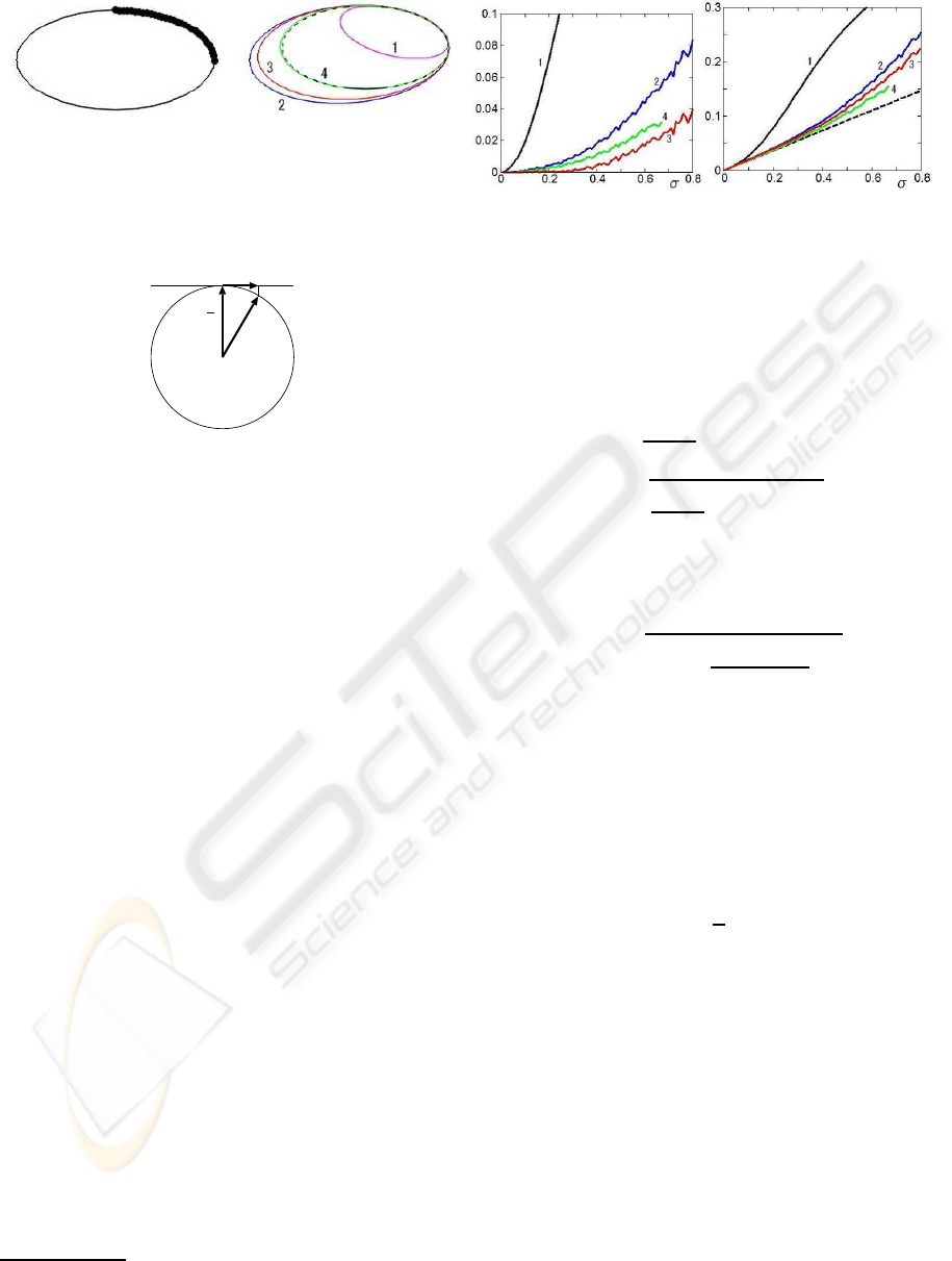
(a) (b)
Figure 1: (a) 31 points on an ellipse. (b) Instances of fitted
ellipses for σ = 0.5. 1. Least squares. 2. Taubin method. 3.
Proposed method. 4. Maximum likelihood. The true shape
is indicated in dashed lines.
θ
∆ θ
θ
O
Figure 2: The true value
¯
θ, the computed value θ, and its
orthogonal component ∆θ to
¯
θ.
their definitions by the observations (x
α
,y
α
). This
does not affect our result, because expectations of
odd-order error terms vanish and hence the error in
Eq. (52) is at most O(σ
4
). Thus, the second order
bias is exactly 0. After the terminology used by Al-
Sharadqah and Chernov (2009) for their circle fitting
method, we call our method using Eq. (51) “hyperac-
curate algebraic fitting”.
7 NUMERICAL EXPERIMENTS
We placed 31 equidistant points in the first quadrant
of the ellipse shown in Fig. 1(a). The major and the
minor axis are 100 and 50 pixel long, respectively.
We added to the x- and y-coordinates of each point
independent Gaussian noise of mean 0 and standard
deviation σ and fitted an ellipse by least squares, the
Taubin method, our proposed method, and maximum
likelihood
4
. Figure 1(b) shows fitted ellipses for some
noise instance of σ = 0.5.
Since the computed and the true values θ and
¯
θ are
both unit vectors, we define their discrepancy ∆θ by
the orthogonal component
∆θ = P
¯
θ
θ, (53)
where P
¯
θ
(≡ I−
¯
θ
¯
θ) is the orthogonal projection ma-
trix along
¯
θ. (Fig. 2). Figures 3(a) and (b) plot for
various σ the bias B and the RMS (root-mean-square)
4
We used the FNS of Chojnacki et al. (2000). See
Kanatani and Sugaya (2007) for the details.
(a) (b)
Figure 3: The bias (a) and the RMS error (b) of the fitting to
the data in Fig. 1(a). The horizontal axis is for the standard
deviation σ of the added noise. 1. Least squares. 2. Taubin
method. 3. Proposed method. 4. Maximum likelihood
(interrupted due to nonconvergence). The dotted line in (b)
shows the KCR lower bound.
error D defined by
B=



1
10000
10000
∑
a=1
∆θ
(a)



,
D=
s
1
10000
10000
∑
a=1
k∆θ
(a)
k
2
, (54)
where θ
(a)
is the solution in the ath trial. The dot-
ted line in Fig. 3(b) shows the KCR lower bound
(Kanatani, 1996; Kanatani, 2008) given by
D
KCR
= σ
s
tr[

N
∑
α=1
¯
ξ
α
¯
ξ
⊤
α
(
¯
θ,V
0
[ξ
α
]
¯
θ)

−
]. (55)
Standard linear algebra routines for solving the
generalized eigenvalue problem in the form of
Eq. (15) assumes that the matrix N is positive defi-
nite. As can be seen from Eq. (17), however, the ma-
trix N
T
for the Taubin method is positive semidefinite
having a row and a column of zeros. The matrix N in
Eq. (51) is not positive definite, either. This causes no
problem, because Eq. (15) can be written as
Nθ =
1
λ
Mθ. (56)
Since the matrix M in Eq. (14) is positive definite for
noisy data, we can solve Eq. (56) instead of Eq. (15),
using a standard routine. If the smallest eigenvalue of
M happens to be 0, it indicates that the data are all ex-
act; any method, e.g., LS, gives an exact solution. For
noisy data, the solution θ is given by the generalized
eigenvector of Eq. (56) for the generalized eigenvalue
1/λ with the largest absolute value.
As we can see from Fig. 3(a), the least square
solution has a large bias, as compared to which the
Taubin solution has a smaller bias, and our solution
has even smaller bias. Since the least squares, the
Taubin, and our solutions all have the same covari-
ance matrix to the leading order, the bias is the deci-
sive factor for their accuracy. This is demonstrated in
VISAPP 2010 - International Conference on Computer Vision Theory and Applications
10

Figure 4: Left: Edge image containing a small elliptic edge
segment (red). Right: Ellipses fitted to 155 edge points
overlaid on the original image. From inner to outer are the
ellipses computed by least squares (pink), Taubin method
(blue), proposed method (red), and maximum likelihood
(green). The proposed and Taubin method compute almost
overlapping ellipses.
Fig. 3(b): The Taubin solution is more accurate than
the least squares, and our solution is even more accu-
rate.
On the other hand, the ML solution, which mini-
mizes the Mahalanobis distance rather than the alge-
braic distance, has a larger bias than our solution, as
shown in Fig. 3(a). Yet, since the covariance matrix
of the ML solution is smaller than Eq. (38) (Kanatani,
2008), it achieves a higher accuracy than our solution,
as shown in Fig. 3(b). However, the ML computation
may not converge in the presence of large noise. In-
deed, the interrupted plots of ML in Figs. 1(a) and (b)
indicate that the iterations did not converge beyond
that noise level. In contrast, our method, like the least
squares and the Taubin method, is algebraic, so the
computation can continue for however large noise.
The left of Fig. 4 is an edge image where a short
elliptic arc (red) is visible. We fitted an ellipse to the
155 consecutive edge points on it by least squares,
the Taubin method, our method, and ML. The right
of Fig. 4 shows the resulting ellipses overlaid on the
original image. We can see that the least squares solu-
tion is very poor, while the Taubin solution is close to
the true shape. Our method and ML are slightly more
accurate, but generally the difference is very small
when the number of points is large and the noise is
small as in this example.
8 CONCLUSIONS
We have presented a new algebraic method for fitting
an ellipse to a point sequence extracted from images.
The method known to be of the highest accuracy is
maximum likelihood, but it requires iterations, which
may not converge in the presence of lage noise. Also,
an appropriate initial must be given. Our proposed
method is algebraic and does not require iterations.
The basic principle is minimization of the alge-
braic distance. However, the solution depends on
what kind of normalization is imposed. We exploited
this freedom and derived a best normalization in such
a way that the resulting solution has no bias up to the
second order, invoking the high order error analysis
of Kanatani (2008). Numerical experiments show that
our method is superior to the Taubin method, also an
algebraic method and known to be very accurate.
ACKNOWLEDGEMENTS
The authors thank Yuuki Iwamoto of Okayama Uni-
versity for his assistance in numerical experiments.
This work was supported in part by the Ministry of
Education, Culture, Sports, Science, and Technology,
Japan, under a Grant in Aid for Scientific Research C
(No. 21500172).
REFERENCES
Albano, R. (1974). Representation of digitized contours in
terms of conics and straight-line segments, Comput.
Graphics Image Process., 3, 23–33.
Al-Sharadqah, A. and Chernov, N. (2009). Error analysis
for circle fitting algorithms, Elec. J. Stat., 3, 886-911.
Bookstein, F. J. (1979). Fitting conic sections to scattered
data, Comput. Graphics Image Process., 9, 56–71.
Chernov, N. and Lesort, C. (2004). Statistical efficiency
of curve fitting algorithms, Comput. Stat. Data Anal.,
47, 713–728.
Chojnacki, W., Brooks, M. J., van den Hengel, A. and
D. Gawley, D. (2000). On the fitting of surfaces to
data with covariances, IEEE Trans. Patt. Anal. Mach.
Intell., 22, 1294–1303.
Cooper, D. B. and Yalabik, N. (1976). On the computa-
tional cost of approximating and recognizing noise-
perturbed straight lines and quadratic arcs in the plane,
IEEE Trans. Computers, 25, 1020–1032.
Fitzgibbon, A., Pilu, M. and Fisher, R. B. (1999). Direct
least square fitting of ellipses, IEEE Trans. Patt. Anal.
Mach. Intell., 21, 476–480.
Gander, W., Golub, H. and Strebel, R. (1995). Least-squares
fitting of circles and ellipses, BIT, 34, 558–578.
Gnanadesikan, R. (1977). Methods for Statistical Data
Analysis of Multivariable Observations (2nd ed.),
Hoboken, NJ: Wiley.
Hartley, R. and Zisserman, A. (2004). Multiple View Geom-
etry in Computer Vision (2nd ed.), Cambridge: Cam-
bridge University Press.
Kanatani, K. (2006). Ellipse fitting with hyperaccuracy, IE-
ICE Trans. Inf. & Syst., E89-D, 2653–2660.
Kanatani, K. (1993). Geometric Computation for Machine
Vision, Oxford: Oxford University Press.
HYPERACCURATE ELLIPSE FITTING WITHOUT ITERATIONS
11

Kanatani, K. (1996). Statistical Optimization for Geomet-
ric Computation: Theory and Practice, Amsterdam:
Elsevier. Reprinted (2005) New York: Dover.
Kanatani, K. (2008). Statistical optimization for geometric
fitting: Theoretical accuracy analysis and high order
error analysis, Int. J. Comp. Vis. 80, 167–188.
Kanatani, K. and Ohta, N. (2004). Automatic detection
of circular objects by ellipse growing, Int. J. Image
Graphics, 4, 35–50.
Kanatani, K. and Sugaya, Y. (2008). Compact algorithm for
strictly ML ellipse fitting, Proc. 19th Int. Conf. Pattern
Recognition, Tampa, FL.
Kanatani, K. and Sugaya, Y. (2007). Performance evalu-
ation of iterative geometric fitting algorithms, Comp.
Stat. Data Anal., 52, 1208–1222.
Leedan, Y. and Meer, P. (2000). Heteroscedastic regression
in computer vision: Problems with bilinear constraint,
Int. J. Comput. Vision., 37, 127–150.
Matei, B. C. and Meer, P. (2006). Estimation of nonlin-
ear errors-in-variables models for computer vision ap-
plications, IEEE Trans. Patt. Anal. Mach. Intell., 28,
1537–1552.
Paton, K. A. (1970). Conic sections in chromosome analy-
sis, Patt. Recog., 2, 39–40.
Rangarajan, P. and Kanatani, K. (2009). Improved algebraic
methods for circle fitting, Elec. J. Stat., 3, 1075–1082.
Rosin, P. L. (1993). A note on the least squares fitting of
ellipses, Patt. Recog. Lett., 14, 799-808.
Rosin, P. L. and West, G. A. W. (1995). Nonparametric
segmentation of curves into various representations,
IEEE. Trans. Patt. Anal. Mach. Intell., 17, 1140-1153.
Taubin, G. (1991). Estimation of planar curves, surfaces,
and non-planar space curves defined by implicit equa-
tions with applications to edge and range image seg-
mentation, IEEE Trans. Patt. Anal. Mach. Intell., 13,
1115–1138.
APPENDIX
The expectation E[∆
1
M
¯
M
−
∆
1
M] is computed as fol-
lows:
E[∆
1
M
¯
M
−
∆
1
M]
=E[
1
N
N
∑
α=1

¯
ξ
α
∆
1
ξ
⊤
α
+ ∆
1
ξ
α
¯
ξ
⊤
α

¯
M
−
1
N
N
∑
β=1

¯
ξ
β
∆
1
ξ
⊤
β
+∆
1
ξ
β
¯
ξ
⊤
β

]
=
1
N
2
N
∑
α,β=1
E[(
¯
ξ
α
∆
1
ξ
⊤
α
+ ∆
1
ξ
α
¯
ξ
⊤
α
)
¯
M
−
(
¯
ξ
β
∆
1
ξ
⊤
β
+∆
1
ξ
β
¯
ξ
⊤
β
)]
=
1
N
2
N
∑
α,β=1
E[
¯
ξ
α
∆
1
ξ
⊤
α
¯
M
−
¯
ξ
β
∆
1
ξ
⊤
β
+
¯
ξ
α
∆
1
ξ
⊤
α
¯
M
−
∆
1
ξ
β
¯
ξ
⊤
β
+∆
1
ξ
α
¯
ξ
⊤
α
¯
M
−
¯
ξ
β
∆
1
ξ
⊤
β
+ ∆
1
ξ
α
¯
ξ
⊤
α
¯
M
−
∆
1
ξ
β
¯
ξ
⊤
β
]
=
1
N
2
N
∑
α,β=1
E[
¯
ξ
α
(∆
1
ξ
α
,
¯
M
−
¯
ξ
β
)∆
1
ξ
⊤
β
+
¯
ξ
α
(∆
1
ξ
α
,
¯
M
−
∆
1
ξ
β
)
¯
ξ
⊤
β
+ ∆
1
ξ
α
(
¯
ξ
α
,
¯
M
−
¯
ξ
β
)∆
1
ξ
⊤
β
+∆
1
ξ
α
(
¯
ξ
α
,
¯
M
−
∆
1
ξ
β
)
¯
ξ
⊤
β
]
=
1
N
2
N
∑
α,β=1
E[(∆
1
ξ
α
,
¯
M
−
¯
ξ
β
)
¯
ξ
α
∆
1
ξ
⊤
β
+(∆
1
ξ
α
,
¯
M
−
∆
1
ξ
β
)
¯
ξ
α
¯
ξ
⊤
β
+ (
¯
ξ
α
,
¯
M
−
¯
ξ
β
)∆
1
ξ
α
∆
1
ξ
⊤
β
+∆
1
ξ
α
(
¯
M
−
∆
1
ξ
β
,
¯
ξ
α
)
¯
ξ
⊤
β
]
=
1
N
2
N
∑
α,β=1
E[
¯
ξ
α
((
¯
M
−
¯
ξ
β
)
⊤
∆
1
ξ
α
)∆
1
ξ
⊤
β
+tr[
¯
M
−
∆
1
ξ
β
∆
1
ξ
⊤
α
]
¯
ξ
α
¯
ξ
⊤
β
+ (
¯
ξ
α
,
¯
M
−
¯
ξ
β
)∆
1
ξ
α
∆
1
ξ
⊤
β
+∆
1
ξ
α
(∆
1
ξ
⊤
β
¯
M
−
¯
ξ
α
)
¯
ξ
⊤
β
]
=
1
N
2
N
∑
α,β=1

¯
ξ
α
¯
ξ
⊤
β
¯
M
−
E[∆
1
ξ
α
∆
1
ξ
⊤
β
]
+tr[
¯
M
−
E[∆
1
ξ
β
∆
1
ξ
⊤
α
]]
¯
ξ
α
¯
ξ
⊤
β
+(
¯
ξ
α
,
¯
M
−
¯
ξ
β
)E[∆
1
ξ
α
∆
1
ξ
⊤
β
]
+E[∆
1
ξ
α
∆
1
ξ
⊤
β
]
¯
M
−
¯
ξ
α
¯
ξ
⊤
β

=
σ
2
N
2
N
∑
α,β=1

¯
ξ
α
¯
ξ
⊤
β
¯
M
−
δ
αβ
V
0
[ξ
α
]
+tr[
¯
M
−
δ
αβ
V
0
[ξ
α
]]
¯
ξ
α
¯
ξ
⊤
β
+(
¯
ξ
α
,
¯
M
−
¯
ξ
β
)δ
αβ
V
0
[ξ
α
]
+δ
αβ
V
0
[ξ
α
]
¯
M
−
¯
ξ
α
¯
ξ
⊤
β

=
σ
2
N
2
N
∑
α=1

¯
ξ
α
¯
ξ
⊤
α
¯
M
−
V
0
[ξ
α
]
+tr[
¯
M
−
V
0
[ξ
α
]]
¯
ξ
α
¯
ξ
⊤
α
+ (
¯
ξ
α
,
¯
M
−
¯
ξ
α
)V
0
[ξ
α
]
+V
0
[ξ
α
]
¯
M
−
¯
ξ
α
¯
ξ
⊤
α

=
σ
2
N
2
N
∑
α=1

tr[
¯
M
−
V
0
[ξ
α
]]
¯
ξ
α
¯
ξ
⊤
α
+ (
¯
ξ
α
,
¯
M
−
¯
ξ
α
)V
0
[ξ
α
]
+2S [V
0
[ξ
α
]
¯
M
−
¯
ξ
α
¯
ξ
⊤
α
]

(57)
VISAPP 2010 - International Conference on Computer Vision Theory and Applications
12