
LANDMARK CONSTELLATION MATCHING FOR PLANETARY
LANDER ABSOLUTE LOCALIZATION
Bach Van Pham, Simon Lacroix, Michel Devy
CNRS, LAAS, 7 Avenue du Colonel Roche, F-31077 Toulouse, France
University of Toulouse, UPS, INSA, INP, ISAE, LAAS, F-31077 Toulouse, France
Marc Drieux
EADS-ASTRIUM, 66 Route de Verneuil, Les Mureaux Cedex, 78133, France
Thomas Voirin
European Space Agency, ESTEC/ESA, Keplerlaan 1, Postbus 299, 2200 AG Noordwijk, The Netherlands
Keywords:
Landmark Constellation, Pinpoint landing, Absolute navigation.
Abstract:
Precise landing position is required for future planetary exploration missions in order to avoid obstacles on the
surface or to get close to scientifically interesting areas. Nevertheless, the current Entry, Descent and Landing
(EDL) technologies are still far from this capability, as the landing point is predicted with a dispersion of
several kilometres. Therefore, research has been conducted to solve this absolute localization problem (also
called “pinpoint landing”), which allows the spacecraft to localize itself within a known reference – namely
orbital imagery. We propose an approach (nicknamed “Landstel”) which relies on Landmark Constellation
matching that gives an alternative to the current solutions and also avoids the drawbacks of existing algorithms.
The fusion of the inertial sensor relative motion estimation and the Landstel global position estimation yields
a better global position estimation and a higher system’s robustness. Position estimation results obtained both
with standalone Landstel and with the fusion of INS-Landstel via a simulator are shown and analysed.
1 INTRODUCTION
Precise landing position is required for future plan-
etary exploration missions in order to avoid obsta-
cles or to get close to scientifically interesting areas.
Nevertheless, the current Entry, Descent and Land-
ing (EDL) technologies are still far from this capa-
bility (Knocke et al., 2004). Therefore, much of re-
search has been conducted to solve this absolute lo-
calization problem, referred to as “pinpoint landing”,
which allows the spacecraft to localize by itself within
a known reference.
Several approaches have been introduced to solve
the pinpoint landing problem using SIFT feature
matching, crater detection and matching, or optic
flow based approach (Trawny et al., 2006; Cheng and
Ansar, 2005; Janscheck et al., 2006). Among these
approaches, the VISINAV (Trawny et al., 2007) sys-
tem can be considered as one of the most promising
solution. The VISINAV system extracts surface land-
marks in the descent image and then matches them to
an ortho-rectified image of the scene. These matched
points are then used either to estimate or update the
spacecraft’s position. The main drawback of the sys-
tem is therefore its high memory requirement due to
the storage of the scene image and the associated dig-
ital elevation map.
The absolute positioning system Landstel (Pham
et al., 2009) is designed to cope with several con-
straints like low memory requirement, hardware im-
plementation facility and illumination change robust-
ness. Landstel uses a camera as its primary sensor,
along with an altimeter and an inertial sensor – with
which the lander is always equipped. Instead of using
the image radiometric information, the Landstel sys-
tem exploits the geometric relationship between point
landmarks. Therefore, the Landstel system can work
with varying illumination conditions, and especially
match landmarks detected in the orbiter imagery and
the lander images. The storage of individual land-
marks (instead of the whole image) also reduces the
267
Van Pham B., Lacroix S., Devy M., Drieux M. and Voirin T. (2010).
LANDMARK CONSTELLATION MATCHING FOR PLANETARY LANDER ABSOLUTE LOCALIZATION.
In Proceedings of the International Conference on Computer Vision Theory and Applications, pages 267-274
DOI: 10.5220/0002815102670274
Copyright
c
SciTePress
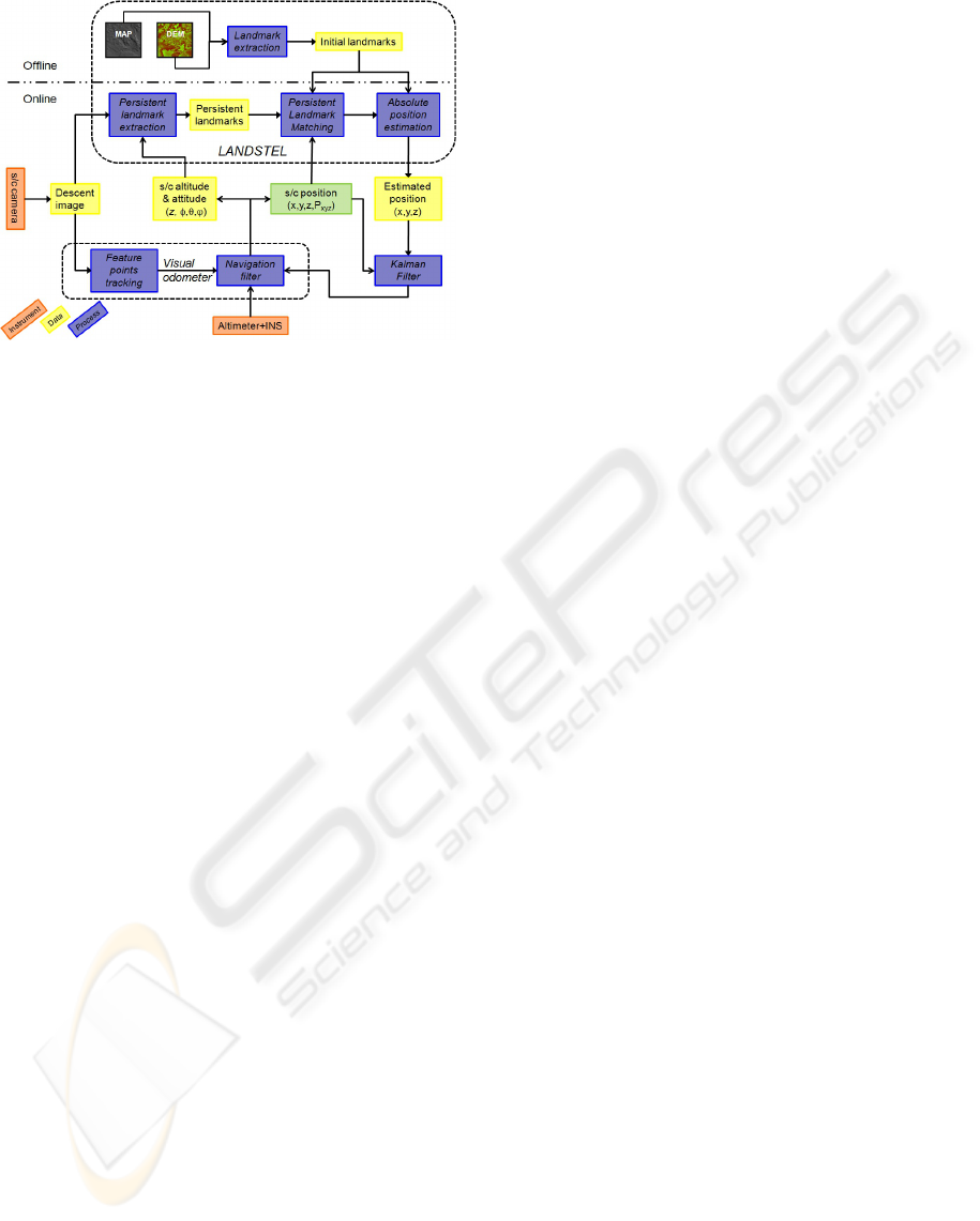
Figure 1: Overall navigation system architecture.
memory requirement for the system.
However, the performance obtained with Lands-
tel in an “standalone” mode doesn’t show the full po-
tential of the whole navigation system (Pham et al.,
2009). Therefore, this paper presents a coupling mode
between Landstel and an INS to define a robust nav-
igation solution. In this coupled system, the INS in-
formation is used to reduce and focus the search area
for the Landstel system, and to compensate the posi-
tion estimation error of Landstel via a complementary
filter.
The next section presents the overall architecture
in which the Landstel system is integrated. The vari-
ous steps involved in the Landstel landmark matching
algorithm are presented in section 3. Then, the paper
presents the approach to fuse the absolute/global po-
sition estimated by Landstel with the relative move-
ment estimated by the INS. Validation result obtained
with standalone Landstel and with the Landstel-INS
coupled system are presented in section 4.
2 OVERALL NAVIGATION
SYSTEM DESCRIPTION
Figure 1 presents the overall navigation system ar-
chitecture with three principle components: the visual
odometer (e.g. like the NPAL camera (Astrium et al.,
2006)) that also integrates INS data, the Landstel sys-
tem and an external Kalman filter. The visual odome-
ter, not described in this paper, provides an estimation
of spacecraft’s velocity and attitude.
The Landstel system is composed of one off-
line and one on-line part. In the off-line part, the
Digital Elevation Map (DEM) and the associated
2D ortho-image (MAP) of the foreseen landing area
(30km × 30km for the current technology (Knocke
et al., 2004)) are obtained on the basis of orbiter im-
agery. Initial visual landmarks are then extracted in
the ortho-image (further denoted as the “geo-image”),
using the Harris feature points detector (Harris and
Stephens, 1988). Depending on the nature of the land-
ing terrain, the appropriate visual landmarks are cho-
sen. A signature is defined for each of the extracted
feature points, according to the process depicted in
section 3. The initial landmarks 2D position, their sig-
nature and their 3D absolute co-ordinates on the sur-
face constitute a database stored in the lander’s mem-
ory before launch.
On-line, the current altitude estimate is exploited
to extract landmarks from the descent images (de-
noted as persistent landmarks in the figure), and the
current spacecraft orientation estimate is used to warp
the landmark coordinates, so as to enable matches
with initial landmarks. Then, the spacecraft abso-
lute position is fused via the Kalman filter with other
available information provided by the visual odome-
ter: speed, orientation, and previous absolute position
estimation.
3 LANSTEL
3.1 Landstel Description
The Landstel algorithm consists in 5 steps (figure 2).
The first and second steps extract and transform the
information in the descent image so that the simi-
larity between the descent landmarks and the initial
landmark is maximized. Then, the third step is used
to extract the signature of each descent landmark.
The extracted signature of each descent landmark is
compared with the initial landmarks signatures (step
4): to each descent landmark is associated a list of
match candidates in the initial landmark set. In the
last step, a voting scheme is applied to asses the cor-
rect matches: several affine transformations are ex-
tracted within the potential candidate list, and the
best affine transformation (the one supported by the
highest number of matches) is used to generate fur-
ther matches between the descent image and the geo-
image.
Step 1 - Landmark Extraction. Unlike the land-
mark extraction method used for geo-image, which
is purely a Harris operator, the landmarks of the de-
scent image are extracted with a scale adjustment op-
erator (Dufournaud et al., 2002). The altimeter input
is used to estimate the scale difference between geo-
image and the descent image.
In fact, the scale-space associated with an image I
can be obtained by convolving the initial image with a
VISAPP 2010 - International Conference on Computer Vision Theory and Applications
268
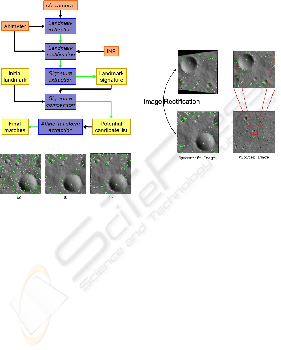
Figure 2: Landstel algorithmaArchitecture.
Figure 3: Landmarks detection with scale adjustment op-
erator (a) Normal operator (b) Scale adjustment operator
(s = 3) (c) Scale adjustment operator (s = 4) on the same
image with added noise.
Gaussian kernel whose standard deviation is increas-
ing monotonically, say sσ with s > 1. In Figure 3,
the two kinds of landmarks that are visible and invisi-
ble from a high altitude are detected in image (a), and
only the ones that are visible from a high altitude are
shown in image (b).
On the one hand, the scale adjustment operator
helps to remove landmarks in the descent-image that
have not been extracted in the geo-image. On the
other hand, it filters the sensor noise thanks to the use
of Gaussian kernel (see image (c) of figure 3, where
the original image has been corrupted with a white
noise N (0,0.01), and with s = 4).
Step 2 - Landmark Rectification. Once extracted
from the descent-image with the scale adjustment op-
erator, the descent landmarks are warped to match the
geo-image orientation with a homography transfor-
mation estimated with the spacecraft orientation pro-
vided by the inertial sensor (Figure 4, left). During
this step, the landing zone is considered as a flat area
due to the long distance between the spacecraft and
the surface. This step will naturally ease the landmark
matching process. Figure 4 right shows that after the
scale adjustment operator and the image warping, the
detected landmarks are pretty well matching those of
the geo-image.
Figure 4: (a) Rectification of descent-image (b) Corre-
sponding zoomed region in geo-image.
Step 3 - Signature Extraction. With the scale ad-
justment, the descent-landmarks have a pixel res-
olution similar to that of landmarks in the geo-
image. The Landstel system uses this property to find
matches between landmarks extracted from these two
images: the signature of the landmark is indeed de-
fined using their relative geometric repartition, mea-
sured using a variation of the Shape Context algo-
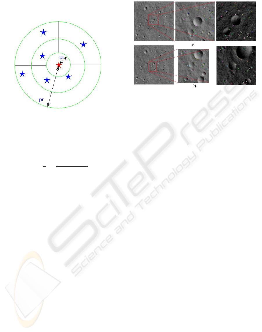
rithm (Belongie and Malik, 2000).
The signature of a landmark L
i
is extracted ac-
cording to the following steps:
1. Determination of Neighbors set: a generic land-
mark L
j
is added to the Neighbors set of L
i
if and
only if its pixelic distance to L
i
, D
i j
, satisfies the
following condition
br < D
i j
< pr (1)
where br is the minimum distance which is used
to prevent noise and pr is the pattern radius.
2. Angular Distances Discretization and Sector Dis-
cretization: the landmarks pixelic distances and
their angular values in the Neighbors set of L
i
are
then discretized into a bi-dimensional nRings ×
nWedges array, corresponding to nRings rings
centered on L
i
and to nWedges sectors (figure 5).
An occupancy histogram, normalized into a prob-
abilistic distribution, defines the signature.
LANDMARK CONSTELLATION MATCHING FOR PLANETARY LANDER ABSOLUTE LOCALIZATION
269
As a result, a landmark signature is a bi-
dimensional vector of nRings × nWedges bytes.
Figure 5: Discretisation used to compute the landmark sig-
nature.
Step 4 - Signature Comparison. In order to calcu-
late the similarity between two landmarks g and k, the
Chi-Square distance C
gk
is used:
C
gh
=
1
2
k
∑
k=1
[g(k) − h(k)]
2
g(k) + h(k)
(2)
Any pair of landmarks whose distance is smaller
than a threshold is considered as a potential match,
which defines for each descent landmark L
i
a list of
potential geo landmark matches.
Step 5 - Affine Transformation Estimation. Given
the candidate lists obtained with the previous steps,
several affine transformations between the descent-
image the geo-image are calculated, each affine trans-
formation defning a number of matches.
The main process used in this step is the interpre-
tation tree and the vector distance metrics. Given two
match pairs (L
i
,K
i
) and (L
j
,K
j
) where L and K re-
spectively represent the descent and geo landmarks,
these pairs are considered as consistent if and only
if their vector distance distVector([L
i
,L
j
],[K
i
,K
j
]),
defined as the difference between the two vectors
lengths and orientations, is smaller than a predefined
threshold ε. This vector distance is meaningful be-
cause the two landmark sets share the same coordinate
system after the application of the affine transforma-
tion (the translation component is not considered in
the vector distance).
On the basis of the vector distance metrics,
an affine transformation (estimated with at least 3
matches) can be estimated by searching an interpreta-
tion tree formed with the candidates lists. If an affine
transformation is found, the associated matches are
Figure 6: Two examples of matches established by Landstel
under different illumination conditions.
stored aside. Other new affine transformations are
searched using remaining other candidates in the po-
tential candidate list.
For each estimated affine transformation, the num-
ber of matches between the descent landmarks and
geo-landmarks are calculated. The affine transforma-
tion with the highest number of matches is used to
generate the final matches between the two images. If
the number of matches is greater than a pre-defined
threshold, the found final matches are considered as
correct and used to estimate the absolute spacecraft’s
position.
3.2 Landstel Illustration
Figures 6 shows two examples of the final matches
with different illumination conditions. The geo-image
(left) is acquired with 55-25 (azimuth-elevation) sun
position, whereas the descent images (right) are ac-
quired at 5710m altitude with 145-10 Sun position (a)
and at 3052m altitude with 235-10 Sun position (b).
The center images show the corresponding matched
regions of the descent-images in the geo-images.
3.3 Absolute Spacecraft Position
Estimation
Given a set of matches between the descent image
and the geo-image, the spacecraft’s position can be
estimated using the image projection function as il-
lustrated in Figure 7:
1. The landmarks 2D positions (U ) in the descent
image
2. The landmarks 3D positions (M) in the land-
ing zone (deduced through their matches with
the geo-image) expressed in a known coordinates
frame
VISAPP 2010 - International Conference on Computer Vision Theory and Applications
270
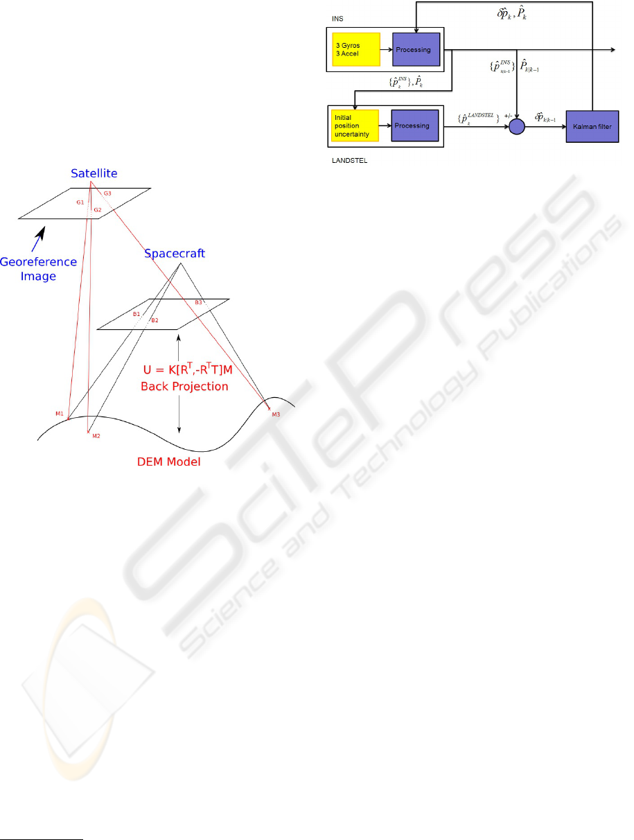
3. The image projection function:
U = K[R
T
,−R
T
T ]M (3)
where K is the 3 × 3 intrinsic matrix of the cam-
era, R the image rotation (provided by the navigation
filter) and T the spacecraft position
1
(Figure 7).
Knowing U, K, R and M, the spacecraft position
T can be calculated using a non-linear optimization
algorithm.
Figure 7: Spacecraft position estimation.
4 KALMAN FILTER
DESCRIPTION
The main objective of fusing the Landstel absolute
position estimates with the relative motion estimates
provided by the INS (or the visual odometry block of
figure 1) is to yield a more precise abolsute estimate
of the spacecraft position. This is achieved thanks to
a complementary filter (a Kalman filter in this case,
set up as shown in Figure 8).
But in turn, the integration of the estimated mo-
tions provided by the INS sensor can help Landstel,
by focusing the match search within a specific region
of the geo-image instead of searching in the whole
landing area, as when using Landstel in a standalone
mode. This focusing mechanism not only accelerates
the algorithm by reducing the search area, but also
improves the algorithm’s performance by limiting the
false matches probability.
1
For simplification purpose, the spacecraft reference
frame is assimilated to the camera one here.
Figure 8: The Landstel-INS fusion principle.
4.1 Kalman Filter Structure
The Kalman filter setup presented in figure 8 is the
following:
1. System state:
x = [δΨ
T
δv
T
δp
T
] (4)
where δΨ is the system attitude error, δv the sys-
tem speed error and δp the system position error.
Each of these is a 3-dimensional vector (3×1). In
this case, the control value is equal to zero : u = 0.
2. Transition matrix:
Φ
k
=
−Ω
e
ie
0
3
0
3
[a×] −2Ω
e
ie
ϒ
0
3
I
3
0
3
(5)
where Ω
e
ie
is a skew-symmetric matrix which rep-
resents the planet rotation given by the angu-
lar rate ω
e
ie
= [ω
1
,ω
2
,ω
3
] between the planet-
centered inertial frame (i-frame) and the planet-
centered planet-fixed frame (e-frame):
Ω
e
ie
=
0 −ω
3
ω
2
ω
3
0 −ω
1
−ω
2
ω
1
0
(6)
and ϒ = −(Ω
e
ie
Ω
e
ie
− Γ
e
), Γ
e
being the short no-
tation for the gravity gradient (the derivative of
the gravity). The 0
3
symbol denotes a 3 × 3 ma-
trix while a I
3
denotes a 3 × 3 identity matrix.
The [a×] represents the misalignment of the trans-
formation matrix between the i-frame and the e-
frame.
3. Observation state: the observations from the
Landstel system are only the spacecraft position.
Hence when a Landstel absolute position estima-
tion becomes available, an error observation is ob-
tained, and the filter then updates the estimate of
the error states in the INS. Otherwise, the system
can use the inertial sensor alone to navigate.
LANDMARK CONSTELLATION MATCHING FOR PLANETARY LANDER ABSOLUTE LOCALIZATION
271
z
k
=
0
2×3
[p
INS
k
− p
Landstel
k
]
(7)
4. Observation matrix:
H
k
=
0 0 0
0 0 0
1 1 1
(8)
4.2 Kalman Filter Design
As the Kalman filter used in the navigation system
is a feed backward filter where the estimated error is
provided to the INS after each observation, the pre-
diction state in this case is always equal to zero. In
fact, initially the inertial sensors are considered as be-
ing calibrated and all the errors are removed, thus the
prediction state x(1|0) is set to zero. Moreover, after
each estimation with the Kalman filter, the estimated
error is always returned back to the INS sensor for
correction due to the feed backward Kalman filter. As
a consequence, the error in the INS sensor is consid-
ered as being corrected which results in a zero predic-
tion state.
The interests of the Kalman filter in this case are
firstly to estimate the error in the estimated position
provided by the INS and also by the previous Kalman
update via the feed backward mechanism. The second
goal of the Kalman filter is to estimate the uncertainty
in the estimated position. The uncertainty of the esti-
mated position can be evaluated through the predicted
covariance matrix
ˆ
P
k|k−1
.
5 RESULTS
5.1 Experiment Profile
The Landstel landmarks matching algorithm has been
tested with the PANGU simulator v2.7 (Parkes et al.,
2004). In this experiment, a simulated trajectory of a
spacecraft during its Mars entry phase is used, from
the early parachute phase to the end of the pow-
ered guidance phase. The spacecraft begins its im-
age acquisition at 8 km altitude with 30 degree incli-
nation (with respect to the vertical axis) and with a
speed of 500m/s. The initial position uncertainty is
15 ×15km
2
. At 2 km altitude, the spacecraft becomes
parallel with the vertical axis with 0 degree inclina-
tion. Then, a propulsion system is used to land the
spacecraft to the ground during 38 seconds. In total,
the whole descent process will take about 65 seconds
from the beginning of the parachute phase to the final
touch down. Therefore, there are 65 images taken for
each trajectory at 1Hz sample rate.
In order to generate more trajectories for the val-
idation process, the simulated trajectory is rotated 30
degrees in the X-Y plane. By this way, 12 different
trajectories are generated. These 12 trajectories begin
the parachute phase at different places and with dif-
ferent angles. The common point of these trajectories
is that they always land the spacecraft in the center of
the image
2
.
The simulated terrain is a heavily craterized sur-
face with about 20 craters/km
2
and has a surface of
32 × 32km
2
.
The descent-image is compared to the geo-image
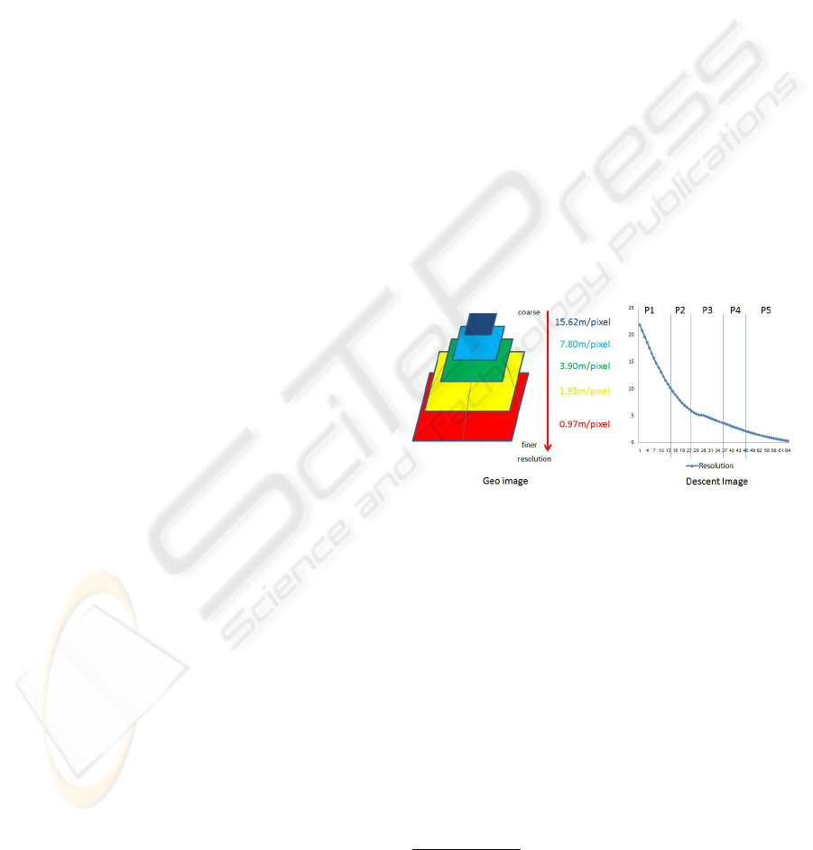
with multiple resolutions as shown figure 9. Since the
spacecraft approaches the surface, the coarseness of
the acquired image is reduced as shown in the right
image. In order to ensure the highest correlation be-
tween the descent-image and the geo-image, the geo-
image layer is changed with respect to different in-
stances as shown in Figure 9. The altitudes a which
the geo-image resolution is switched are predefined.
Figure 9: Multi-resolution geo-image.
Since the geo-image is taken under illumination
conditions which can be different from the conditions
as the spacecraft descends, different illumination con-
ditions are used to verify the robustness of the system.
Here, the geo-image illumination condition is fixed to
0-5 degrees azimuth-elevation. The conditions dur-
ing the spacecraft descent vary as indicated in table 1.
The first number is each bracket is the azimuth value
which is an increment of 40 degrees and the second
number indicates the elevation value which is either
1 degree or 10 degrees. Therefore, there are 18 dif-
ferent illumination conditions used. In summary, the
18 different illuminations combined with the 12 dif-
ferent trajectories generate 216 test cases (or ”trials”),
2
This is due to the way Pangu handles large terrain mod-
els – the higher resolution being only available in the center
of the model.
VISAPP 2010 - International Conference on Computer Vision Theory and Applications
272
i.e. 14040 images in total
3
.
Table 1: Descent image illumination conditions.
(00,01) (40,01) ... (280,01) (320,01)
(00,10) (40,10) ... (280,10) (320,10)
In order to verify the robustness of the system with
different levels of sensor noise, the experiment is set
up with the following configuration:
1. Image: white noise N (0, 0.005)
2. Radar altimeter: 2.5 percent of measured distance
(e.g. 5000m altitude with ±125m error).
3. Attitude noise: the INS is considered as extremely
precise due to the short landing time and the usage
of the visual odometer (standard deviation well
below 1
◦
– the Landstel has however shown to be
able to cope with 5
◦
attitude angle errors (Pham
et al., 2009)).
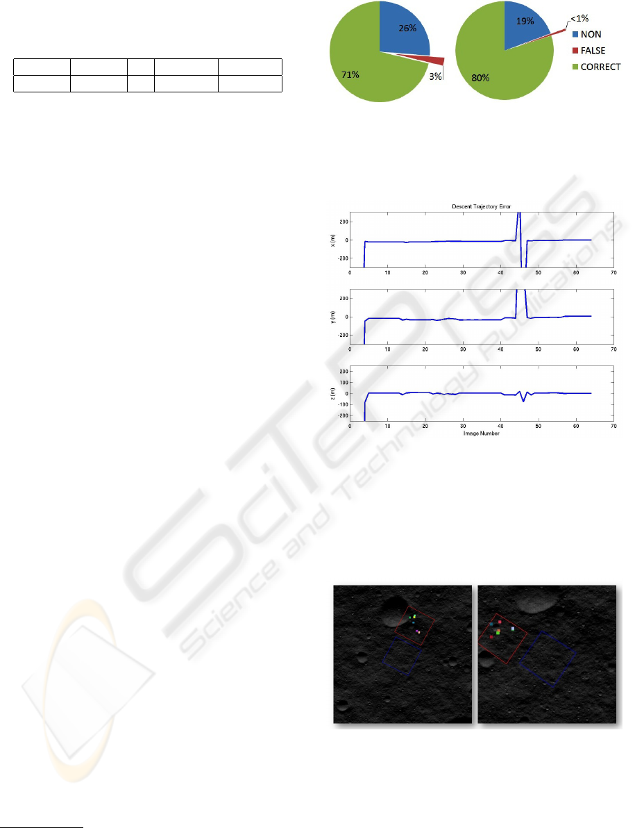
5.2 System Performance
5.2.1 Overall Performance
Figure 10 shows the estimation results obtained. As
shown in the two charts, the combination of the iner-
tial sensor and the Landstel system shows better per-
formance than Landstel in a standalone mode. In this
case, the number of ”no estimation” is decreased from
26 percent down to 19 percent. Moreover, the number
of ”false estimations” is also decreased from 3 percent
down to less than 1 percent (105 false estimations in
14040 cases). As a consequence, the number of cor-
rect estimations is increased from 71 percent up to 80
percent. Concerning the false estimations delivered
by the INS-Landstel fusion, most of the cases happen
at the end of each geo-image layer transition where
the correlation between the descent image resolution
and the geo-image layer becomes weak.
5.2.2 Localization Performance
In general, from the initial 15 × 15 k m
2
uncertainty,
both of the standalone Landstel and the INS-Landstel
systems can localize the spacecraft’s position with a
precision below 10 × 10 m
2
at the final touch down.
However, the difference between the two systems
is the number of false position estimations which
can severely influence the whole spacecraft’s perfor-
mance.
3
Dozens of similar tests with different terrain configura-
tions, yieding the same number of images, have also been
evaluated.
Figure 10: Estimation result with the number of ”False” and
“correct” estimations, and the number of images where the
algorithm can not find matches. The left chart shows the re-
sults obtained with Landstel in a standalone mode, the right
one shows the result obtained with INS-Landstel fusion.
Figure 11: Estimation error with standalone Landstel.
Figure 11 shows for one trial the difference be-
tween the the estimated position returned by stan-
dalone Landstel and the true spacecraft trajectory.
The sun condition in this trial is 180 degrees in az-
imuth and 1 degree in elevation for the descent-image.
Figure 12: Two false position estimations situations with
standalone Landstel. The red zone indicates the estimated
the spacecraft’s camera’s field of view, whilst the blue zone
indicates the true spacecraft’s camera’s field of view.
In this trial, the standalone Landstel system re-
turns two false estimations which occur at the 45
th
and the 46
th
images, which results in two big error
jumps as shown in Figure 11. The two erroneous
LANDMARK CONSTELLATION MATCHING FOR PLANETARY LANDER ABSOLUTE LOCALIZATION
273
cases are shown in Figure 12. In this Figure, the
shown images are the cropped zones of the geo-image
in order to enhance the visibility. However, the im-
ages’ intensity is not changed so as to reflect the true
illumination condition of the geo-image.
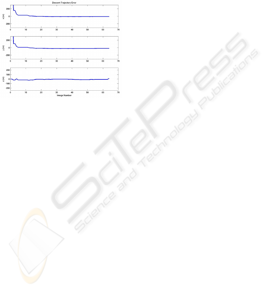
Figure 13: Estimation error with the INS-Landstel fusion.
In contrast, with the same trial, the INS-Landstel
fusion can avoid these two errors as shown in Figure
13. With the motion estimation of the inertial sen-
sor, the research zone within the geo-image is well
focused, which reduces the probability of false match-
ing occurrences.
6 CONCLUSIONS
In this paper, we have demonstrated the ability of a
vision-based algorithm coupled with the inertial sen-
sor for spacecraft absolute localization with respect
to an orbiter image. Similarly to an INS-GPS fusion
problem, the advantages obtained are twofold. Firstly,
the localization precision is higher. Secondly, the re-
search zone within the geo-image for the Landstel al-
gorithm is greatly reduced, which both enhances the
algorithm’s speed and reduces the probability of false
matches.
However, the fusion mechanism introduced in this
paper only exchanges the position (both global and
relative) information of the two sensors. A tighter in-
tegration of the two sensors with respect to the inter-
est points detected by both sensors is currently being
analysed and evaluated. First results have shown a
promising application of this type of integration.
REFERENCES
Astrium, E., Avionica, G., of Dundee, U., INETI, and
SCISYS (2006). Navigation for planetary approach
& landing. ESA Contract.
Belongie, S. and Malik, J. (2000). Matching with shape
context. IEEE Workshop on Context Based Access of
Image and Video Libraries.
Cheng, Y. and Ansar, A. (2005). Landmark based posi-
tion estimation for pinpoint landing on mars. Pro-
ceedings of the 2005 IEEE International Conference
on Robotics and Automation, pages 1573 – 1578.
Dufournaud, Y., Schmid, C., and Horaud, R. (2002). Image
matching with scale adjustment. INRIA Report.
Harris, C. and Stephens, M. (1988). A combined corner
and edge detector. Proceedings of the 4th Alvey Vision
Conference.
Janscheck, K., Techernykh, V., and Beck, M. (2006). Per-
formance analysis for visual planetary landing navi-
gation using optical flow and dem matching. AIAA
Guidance, Navigation and Control.
Knocke, P. C., Wawrzyniak, G. G., Kennedy, B. M., and
Parker, T. J. (2004). Mars exploration rovers landing
dispersion analysis. AIAA/AAS Astrodynamics Spe-
cialist Conference and Exhibit.
Parkes, S., Martin, I., Dunstan, M., and Matthews,
D. (2004). Planet surface simulation with pangu.
SpaceOps.
Pham, B. V., Lacroix, S., Devy, M., Drieux, M., and
Philippe, C. (2009). Visual landmark constellation
matching for spacecraft pinpoint landing. AIAA Guid-
ance, Navigation and Control.
Trawny, N., Mourikis, A. I., and Roumeliotis, S. I. (2007).
Coupled vision and inertial navigation for pin-point
landing. NASA Science Technology Conference.
Trawny, N., Mourikis, A. I., Roumeliotis, S. I., Johnson,
A. E., and Montgomery, J. (2006). Vision-aided in-
ertial navigation for pin-point landing using obser-
vations for mapped landmarks. Journal of Fields
Robotics.
VISAPP 2010 - International Conference on Computer Vision Theory and Applications
274
