
A
UTOMATIC CONSTRUCTION OF HIERARCHICAL HIDDEN
MARKOV MODEL STRUCTURE FOR DISCOVERING SEMANTIC
PATTERNS IN MOTION DATA
O. Samko, A. D. Marshall and P. L. Rosin
School of Computer Science, Cardiff University, Cardiff, U.K.
Keywords:
HHMM structure, Pattern recognition, Motion analysis.
Abstract:
The objective of this paper is to automatically build a Hierarchical Hidden Markov Model (HHMM) (Fine
et al., 1998) structure to detect semantic patterns from data with an unknown structure by exploring the natural
hierarchical decomposition embedded in the data. The problem is important for effective motion data repre-
sentation and analysis in a variety of applications: film and game making, military, entertainment, sport and
medicine. We propose to represent the patterns of the data as an HHMM built utilising a two-stage learning al-
gorithm. The novelty of our method is that it is the first fully automated approach to build an HHMM structure
for motion data. Experimental results on different motion features (3D and angular pose coordinates, silhou-
ettes extracted from the video sequence) demonstrate the approach is effective at automatically constructing
efficient HHMM with a structure which naturally represents the underlying motion that allows for accurate
modelling of the data for applications such as tracking and motion resynthesis.
1 INTRODUCTION
Hierarchical Hidden Markov Models (HHMMs)
(Fine et al., 1998) have become popular for modelling
real world data which have non-linear variations and
underlying hierarchical structure. This form of mod-
elling has been found useful in applications such as
handwritten character recognition (Fine et al., 1998),
activity recognition (Kawanaka et al., 2006), (Nguyen
and Venkatesh, 2008) and DNA sequence analysis
(Choi et al., 2009), (Hu et al., 2000).
The automatic discovery of an HHMM topol-
ogy from original data is an important yet compli-
cated problem. This has not to date gained that
much attention; some work in this area has been re-
ported in (Xie et al., 2003), (Youngblood and Cook,
2007). The structure discovery algorithm by Xie (Xie
et al., 2003) employs the Markov Chain Monte Carlo
(MCMC) method to determine structure parameters
for an HHMM in an unsupervised manner. This ap-
proach is used to discover patterns in video, namely
play and break, and is based on a bespoke proce-
dure to select features from the video. Youngblood
and Cook (Youngblood and Cook, 2007) examine the
problem of automatic learning of a human inhabitant
behavoural model. They extract sequential patterns
from inhabitant activities using the Episode Discov-
ery (ED) sequence mining algorithm. An HHMM is
created using low-level state information and high-
level sequential patterns. This is used to learn an ac-
tion policy for the environment. This model, as with
(Xie et al., 2003), was developed to represent specific
features inherent in the data.
We propose the algorithm, constructed with
the non-linear dimensionality reduction approach,
Isomap (Tenenbaum et al., 2000), and based on
Isomap’s ability to preserve data geometry at all
scales (Silva and Tenenbaum, 2003). Using this prop-
erty, we can explore the data trajectory in the em-
bedded space. We also employ the assumption of
the motion data trajectory smoothness during analy-
sis of the space. Under these conditions we propose
that by utilising hierarchical clustering we can con-
struct an HHMM topological structure in the Isomap
space, and the obtained HHMM is efficient in explor-
ing semantic patterns in the motion data. We build
an HHMM using our algorithm and learn the model
with Dynamic Bayesian Network (DBN) (Murphy
and Paskin, 2001). After the model training, we test it
by exploring observed motion patterns from the new
unseen data.
275
Samko O., D. Marshall A. and L. Rosin P. (2010).
AUTOMATIC CONSTRUCTION OF HIERARCHICAL HIDDEN MARKOV MODEL STRUCTURE FOR DISCOVERING SEMANTIC PATTERNS IN
MOTION DATA.
In Proceedings of the International Conference on Computer Vision Theory and Applications, pages 275-280
DOI: 10.5220/0002815202750280
Copyright
c
SciTePress
We investigate the first stage of data process-
ing, hierarchical content characterisation algorithm,
in Section 2. In Section 3, we automatically con-
struct a dynamic model for semantic pattern discov-
ery using parameters obtained at the first stage. Sec-
tion 4 demonstrates the effectiveness of our algorithm
by applying it to the different motion data features,
namely silhouettes, 3D coordinates and angular (Ac-
claim) data. Conclusion and future work are given in
Section 5.
2 HIERARCHY CONSTRUCTION
The algorithm’s first stage consists of three main
steps, described below in separate subsections. The
algorithm is generic, in that it is able to work with
various unlabelled feature sequences, extracted from
the original motion data. Also we assume that the data
is complete, i.e. without missing (unobserved) values.
2.1 Trajectory Extraction
Isomap, as a manifold learning technique, represents
global data relationships in a low dimensional space,
maximally preserving geodesic distances between all
pairs of data points (Tenenbaum et al., 2000). We em-
ploy this Isomap ability and represent an input data as
a point-wise trajectory in an embedded space for the
initial data analysis.
The basic idea of the Isomap algorithm is to use
geodesic distances on a neighborhood graph in the
framework of the Multidimensional scaling (MDS)
algorithm. The success of Isomap in the data repre-
sentation and model accuracy depends on being able
to choose an appropriate neighborhood size. We use
the method for automatic selection of this parameter
described in (Samko et al., 2006).
2.2 GMM on the Embedded Space
The Gaussian Mixture Model (GMM) is a flexible
and powerful method for unsupervised data grouping
(McLachlan and Basford, 1988). In addition to group-
ing, it gives us parameters which we use to initialise
our dynamic model at the second stage of the data
processing.
To choose the number of Gaussian clusters we use
the method described in (Bowden, 2000). Accord-
ing to this method, the Characteristic Cost Graph is
produced and the optimal number of clusters is deter-
mined by locating a point where increasing the num-
ber of clusters does not lead to a significant decrease
in the resulting cost. We perform a more accurate es-
timation of that point with the procedure for threshold
estimation (Rosin, 2001).
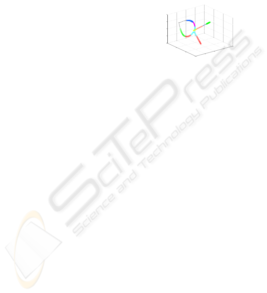
Figure 1 shows an example of Gaussian clustering
in the Isomap space. The data points form a trajectory
which represents the original data sequence.
−4000
−2000
0
2000
4000
−2000
−1000
0
1000
−1000
−500
0
500
1000
Figure 1: GMM clustering (10 clusters) of the walking data
in Isomap space.
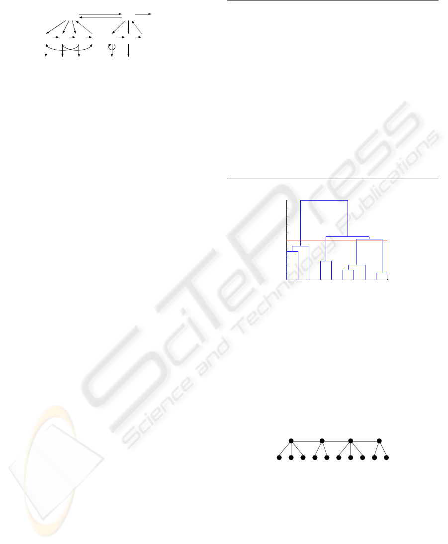
2.3 Hierarchical Data Organisation
To construct a hierarchy over the obtained clusters,
we employ the standard agglomerative clustering al-
gorithm (Duda et al., 2000) because this approach at-
tempts to place the input elements in a hierarchy in
which the distance within the tree reflects similarity
between the elements. As an input, we use means
of the Gaussian clusters. The result of the hierarchi-
cal clustering is represented as a dendrogram tree, see
Figure 3 for example.
3 DYNAMIC PATTERNS
DISCOVERY
Using the hierarchy constructed in the previous sec-
tion as a basis, we now aim to construct a two-level
HHMM which considers parts of motion as separate
submodels. The top HHMM level corresponds to the
main actions in the motion data, and at the bottom the
initial data sequence is divided into subsequences ac-
cording to the actions they represent. The choice of
the number of levels is natural: every data sequence
has at least a single pattern (subsequence), while hav-
ing more levels could be unnecessary for many appli-
cations as well as being computationally expensive.
3.1 HHMM Definition
An HHMM forms a hierarchy of HMMs, where a top
level HMM can have sub HMMs as its hidden nodes.
Figure 2 shows an example of the HHMM state transi-
tion diagram, which consists of two HMMs with three
VISAPP 2010 - International Conference on Computer Vision Theory and Applications
276
and two states at the bottom level, and one two-state
HMM at the top level.
Q
Q Q Q Q Q
e
e
e
O
O
O
O
O
Q
1
1
1
2
2
1
2
2
2
3
2
1
2
2
Figure 2: A two-level HHMM with observations at the bot-
tom. Black edges denote vertical and horizontal transitions
between states and observations O. Dashed edges denote re-
turns from the end state of each level e to the level’s parent
state Q
d
t
(t is the state index, d is the hierarchy level).
A full HHMM is defined as a 3-tuple
H =< λ, ζ, Σ > (1)
Here λ is a set of parameters, ζ is the topological
structure of the model, and Σ is an observation alpha-
bet. The set of parameters λ consists of a horizontal
transition matrix A, mapping the transition probability
between child nodes of the same parent; an observa-
tion probability distribution B and a vertical transition
vector Π that assigns the transition probability from a
hidden node to its child nodes:
λ =< A, B, Π > (2)
The topology ζ specifies the number of levels, the
state space at each level, and the parent-children re-
lationship between levels. The states include “pro-
duction states” that emit observations and “abstract
states” which are hidden states. The observation al-
phabet Σ consists of all possible observation finite
strings.
3.2 HHMM Structure Construction
In an HHMM, every higher-level state corresponds to
a stream produced by lower-level sub-states, a transi-
tion at the top level is invoked only when the lower-
level HMM enters an exit state. Therefore it is natural
to construct an HHMM in a “bottom-up” manner.
After the hierarchical clustering algorithm is ap-
plied to the initial data, we get the data dendrogram
representation as in Figure 3. We use this represen-
tation to construct the HHMM structure. The pro-
posed HHMM structure construction algorithm out-
line is presented in Table 1.
We apply a heuristic approach for construction of
the HHMM structure: we cut the dendrogram using
the mean distance between clusters measure, and use
the clustering specified by the dendrogram at that cut-
off level. The purpose of this is to provide clusters
that are similar enough to be grouped together, and
Table 1: An automatic HHMM structure construction algo-
rithm.
1. Find the dendrogram cut-off level using the mean
distance between clusters. Remove all dendro-
gram levels above the cut-off and intermediate
levels between this level and the bottom dendro-
gram level. Label nodes.
2. Set the top-HMM number of states and number
of bottom-HMMs equal to the number of clusters
at the cut-off level. Set the number of bottom-
HMMs states equal to the number of clusters in
the corresponding dendrogram branches.
3. Identify transitions between the states using
GMM labels. Set a transition between the states
Q
i
and Q
j
if there exist successive points from
the data sequence y
t
, y
t+1
such that y
t
∈ Q
i
and
y
t+1
∈ Q
j
.
0
500
1000
1500
2000
2500
3000
3500
4000
4500
5000
Data index
Distance
Dendrogram
1 8 9 2 10 3 7
5 4 6
Figure 3: A dendrogram for the walking data. The red line
indicates the cut-off level. Four clusters at the top level are
formed in this example.
the sizes of these groups are large enough to construct
a regular HMM with them. Figure 4 illustrates the hi-
erarchy for the motion data, obtained from the den-
drogram shown in Figure 3. Using this representation
we set the number of states for each HMM (for this
particular example these numbers are 4 for the top-
HMM, and 3, 2, 3 and 2 for the bottom level HMMs).
1 8 9 2 10 3 7 5 4 6
11 12 13 14
Figure 4: A hierarchical representation for the motion data.
Figure 5 shows the resulting HHMM structure (ζ
from Equation 1) - state transition diagram. Black
arrows denote state transitions, and dotted arrows de-
note returns to the parents states. Our HHMM does
not have a fully connected topology because we lim-
ited the transitions by using the GMM labels obtained
at the first stage. This reduces the number of transi-
tion matrix non-zero elements and simplifies calcula-
tion of the HHMM parameters.
AUTOMATIC CONSTRUCTION OF HIERARCHICAL HIDDEN MARKOV MODEL STRUCTURE FOR
DISCOVERING SEMANTIC PATTERNS IN MOTION DATA
277

5 3 7 2 10 6 4 9 1 8
13 12 14 11
Figure 5: An HHMM state transition diagram for the mo-
tion data.
3.3 Learning HHMM Parameters
To determine the HHMM fully, we need to set λ from
Equation 2. We convert an HHMM into a DBN, to
reduce the time complexity of computation, and learn
the DBN parameters instead to find the parameters of
Equation 2. We use standard DBN parameter learn-
ing procedures, which are best described in (Murphy
and Paskin, 2001). To initialise the model, we use the
GMM parameters from the previous section.
4 EXPERIMENTS
Now we evaluate how the proposed algorithm pro-
cesses different types of motion data, represented by
3D coordinates, angular coordinates and silhouettes
extracted from the video sequences. The data we use
contains a wide range of variation both in upper and
lower body parts, and sequences from several hun-
dreds to several thousands of frames. In Section 4.1,
we extract semantic patterns and evaluate the model
for a gymnastic exercise sequence from the CMU mo-
tion capture (MoCap) database
1
, where motion fea-
tures are represented by 3D angular coordinates. In
Section 4.2 we address the model’s classification abil-
ity with 3D coordinates of a walking person. And
finally, the model is constructed with silhouette se-
quences from the IXMAS motion database
2
.
4.1 CMU MoCap Data
The algorithm input data here is represented by 32
angular coordinates (the video preprocessing and fea-
ture extraction details can be found on the CMU web-
site). This motion data sequence consists of 5357
frames, and contains 8 exercises: jumps, jog, squats,
side twists, lateral bending, side stretch, forward-
backward stretch and forward stretch. In this example
we demonstrate that our method is able to work with
a variety of movements, as well as with long data se-
quences.
We reduce the dimensionality of the original space
to 3 using the automatic method (Samko et al., 2006),
1
http://mocap.cs.cmu.edu
2
http://perception.inrialpes.fr
and perform clustering. In our experiments we as-
sume that motion data has smooth transformations
between points in the embedded space and there-
fore clusters include chains of the neighbour elements
from the original data sequence, i.e. data subse-
quences. Also note that in the Isomap space similar
clusters are close to each other; we use this property
in our model construction.
Figure 6 shows a schematic representation of the
HHMM structure obtained by our algorithm. Each
hidden state here is illustrated by the mean pose for
that state. This Figure shows that we are able to ex-
tract the above mentioned main patterns from the un-
labelled data. There are six states at the top HMM,
which represent jumps, jog, squats, side twists, lat-
eral bending and stretches. At the bottom level we get
six HMMs whose number of states range from two
(squats HMM: down and up states) to seven (lateral
bending). The stretches sub-HMM consists of five
states and represents three exercises at once: side,
forward-backward and forward stretches.
To test the model we take another fragment of
swordplay motion, which consists of 2300 frames and
includes jumps, jog, squats and side twists exercises.
We project the test data into Isomap space using the
kernel function given in (Bengio et al., 2004) and clas-
sify it with our model.
The pattern with the maximum probability is used
to label the data. To verify the result and make a com-
parison with other methods, we manually label train
data with these patterns. We consider this labelling
as a ground truth, and perform classification evalu-
ation with our semi-supervised model, unsupervised
HHMM and flat HMM over the test data. We use the
same structure for the unsupervised HHMM obtained
from our hierarchical algorithm, but without param-
eters initialisation from the algorithm first stage, and
the HMM consisted of the bottom level states of our
model. The classification results are shown in the first
column of Table 2. Using our semi-supervised algo-
rithm, we get better accuracy than the other methods.
An example of state of the art results, (Junejo et al.,
2008) recently reported the average recognition ac-
curacy 91.98% for the pre-defined actions from the
CMU MoCap database. The achieved accuracy shows
the potential advantage of our method in automatic
action recognition.
4.2 Walking Data
We use the sequence of 218 frames which represents
motion of a walking person, consisting of two steps,
right turn and another step. The initial feature param-
eters represent the coordinates of human (arms, legs,
VISAPP 2010 - International Conference on Computer Vision Theory and Applications
278
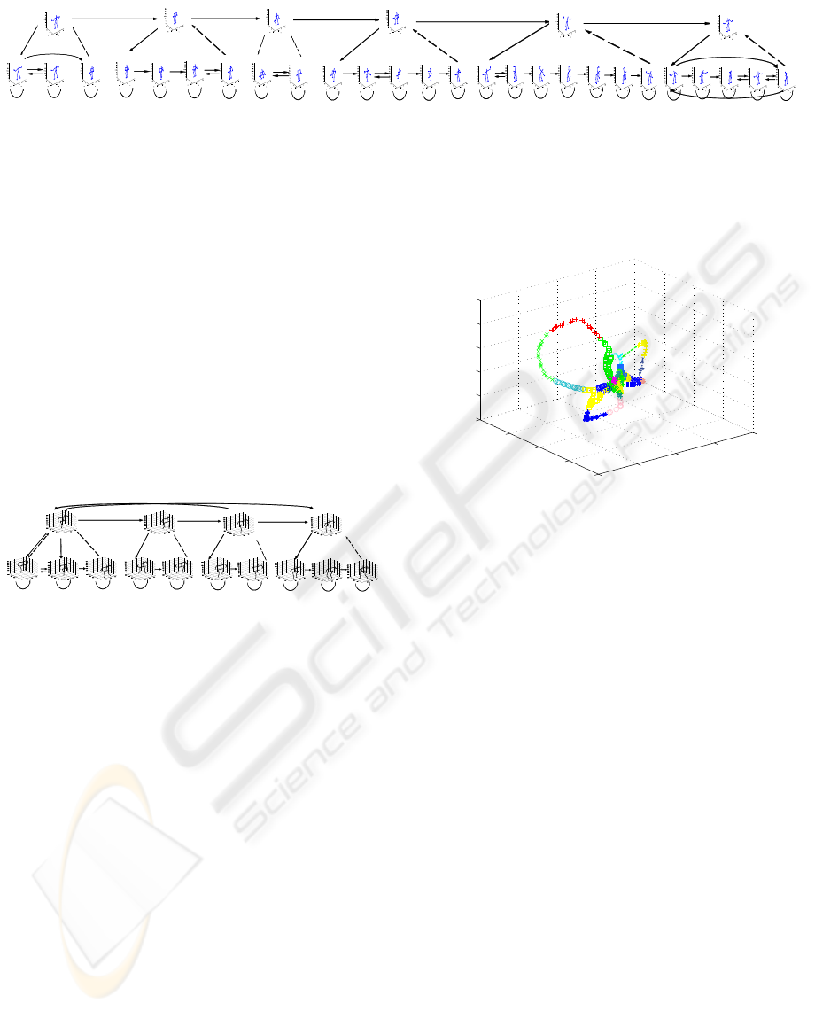
Figure 6: An HHMM state transition diagram for the exercise data.
torso) in the 3D space. Each pose is characterised by
17 points on the body.
We showed some intermediate results for this ex-
ample to illustrate the algorithm in Figures 1, 3, 4.
The HHMM structure is presented in Figure 5 and
Figure 7. We get one top level HMM, which includes
four sub-HMMs. “5-3-7”-states HMM correspond to
the pattern which represents the motion beginning and
start of the turn. “2-10” HMM corresponds to the
sequence pattern with left leg moving down and the
right leg lifting up motions. “6-4”-state HMM move-
ment is opposite to the previous pattern: the right leg
moving down and the left leg lifting up. Finally, “9-
1-8” HMM represents the turn and step after turn pat-
tern. Thus the automatically constructed HHMM ex-
tracts “natural” units from the original data.
Figure 7: An HHMM state transition diagram for the walk-
ing data.
The results of classification are shown in the sec-
ond column of Table 2. We can say that our semi-
supervised HHMM is able to correctly identify the se-
mantic patterns in the test data and classify the motion
patterns better than other methods.
4.3 IXMAS Data
The INRIA Xmas Motion Acquisition (IXMAS) se-
quence we used here contains 11 actions: check
watch, cross arms, scratch head, yoga, turn around,
walk, wave, punch, kick, point and throw away. The
silhouettes were extracted from the video using a stan-
dard background subtraction technique, modelling
each pixel as a Gaussian in RGB space.
Although raw silhouette pixels are not the opti-
mal feature for motion analysis, we use it to show the
algorithm’s ability to work with such difficult input
data. For the Isomap algorithm, it is much harder to
extract main motion features from silhouettes, to em-
bed them into the low dimensional space, and to pro-
duce useful trajectories for further analysis. Isomap
space for the silhouette data is more knotted than for
the coordinate data, which makes clustering and pat-
tern extraction more difficult. Figure 8 illustrates the
embedded space for this example.
−0.4
−0.2
0
0.2
0.4
−0.4
−0.2
0
0.2
0.4
−0.2
−0.1
0
0.1
0.2
0.3
Figure 8: GMM clustering of the IXMAS data in embedded
space.
To test the algorithm we take the sequence of 1076
frames from the IXMAS database. It shows the front
view silhouettes of the person performing the above
actions in the above order.
Figure 9 shows the HHMM structure obtained by
our algorithm. In comparison to the coordinate data,
we get more transitions between the states (because
of the space knotting). As shown in this Figure, the
algorithm recognised five patterns in this data. The
first pattern represents hand movements from a stand-
ing position and includes check watch, cross arms,
scratch head and wave actions. The second pattern
is the yoga action. The next recognised pattern is leg
movements and includes turn around, walk and kick
actions. The fourth pattern is hand movements with
legs apart, this contains punch and point actions. And
the last pattern is the throw away action.
We use another sequence of similar length to test
the model. The classification results are shown in
the last column of Table 2. The accuracy is lower
compared with our earlier experiments because of the
increased complexity of its trajectory in the Isomap
space, but it can be seen that our algorithm is able
to find the meaningful patterns even from such data.
Also it is comparable to the result reported by (Junejo
et al., 2008) for the pre-defined actions from this data
AUTOMATIC CONSTRUCTION OF HIERARCHICAL HIDDEN MARKOV MODEL STRUCTURE FOR
DISCOVERING SEMANTIC PATTERNS IN MOTION DATA
279
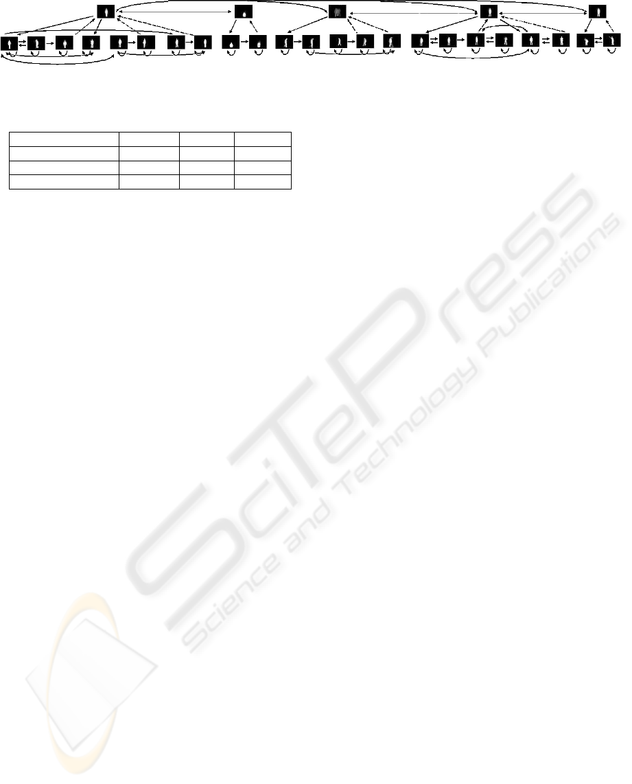
Figure 9: An HHMM state transition diagram for the IXMAS data.
Table 2: Classification results (rate of correct classification).
Method Exercise Walk IXMAS
Semi-sup. HHMM 93.57% 96.95% 71.63%
Unsuperv. HHMM 91.13% 93.13% 65.43%
Flat HMM 90.65% 92.37% 65.43%
set (72.5%), taking into account that we do not make
any manual settings.
5 CONCLUSIONS
We have presented a novel method for the automatic
discovery of an HHMM topological structure applied
to finding semantic patterns in an unlabelled motion
sequence. We demonstrated our algorithm’s ability
to work with various data features obtained from dif-
ferent types of mocap/video sources. Since the al-
gorithm is not linked with any a priori information
from the data, it could be used with various data types
(for example, in DNA sequence analysis). Our algo-
rithm is fully automated with no additional configura-
tion parameters required.
In order to develop a more detailed knowledge of
the strengths and robustness of our algorithm, a more
thorough experimental evaluation of our system will
be carried out in future work. We hope to improve the
robustness and compactness of our model by using al-
ternative clustering algorithms, and we plan to involve
probability estimation to the cut-off level detection.
REFERENCES
Bengio, Y., Paiement, J., and Vincent, P. (2004). Out-
of-sample extensions for LLE, Isomap, MDS, Eigen-
maps and spectral clustering. Advances in Neural In-
formation Processing Systems 16.
Bowden, R. (2000). Learning non-linear models of shape
and motion. PhD Thesis, Dept Systems Engineering,
Brunel University.
Choi, H., Nesvizhskii, A., Ghosh, D., and Qin, Z. (2009).
Hierarchical HMM with application to joint analy-
sis of ChIP-seq and ChIP-chip data. Bioinformatics,
(25):1715–1721.
Duda, R. O., Hart, P. E., and Stork, D. G. (2000). Pattern
classification. Wiley-Interscience Publication.
Fine, S., Singer, Y., and Tishby, N. (1998). The Hierarchi-
cal Hidden Markov Model: Analysis and applications.
Machine Learning, 32(1):41–62.
Hu, M., Ingram, C., Sirski, M., Pal, C., Swamy, S., and Pat-
ten, C. (2000). A hierarchical HMM implementation
for vertebrate gene splice site prediction. Technical
report, Dept. of Computer Science, University of Wa-
terloo.
Junejo, I., Dexter, E., Laptev, I., and Perez, P. (2008).
Cross-view action recognition from temporal self-
similarities. ECCV, pages 293–306.
Kawanaka, D., Okatani, T., and Deguchi, K. (2006).
HHMM based recognition of human activity. IEICE
Transactions Inf. and Syst., 89(7):2180–2185.
McLachlan, G. and Basford, K. (1988). Mixture mod-
els: Inference and applications to clustering. Marcel
Dekker.
Murphy, K. and Paskin, M. (2001). Linear time inference in
Hierarchical HMMs. Proc. Neural Information Pro-
cessing Systems.
Nguyen, N. and Venkatesh, S. (2008). Discovery of activ-
ity structures using the Hierarchical Hidden Markov
Model. BMVC, pages 112–122.
Rosin, P. L. (2001). Unimodal thresholding. Pattern Recog-
nition, 34:2083–2096.
Samko, O., Marshall, A., and Rosin, P. (2006). Selection of
the optimal parameter value for the isomap algorithm.
Pattern Rocognition Letters, 27:968–979.
Silva, V. and Tenenbaum, J. (2003). Local versus global
methods for nonlinear dimensionality reduction. In
Advances in Neural Information Processing Systems,
volume 15.
Tenenbaum, J., Silva, V., and Langford, J. (2000). A global
geometric framework for nonlinear dimensionality re-
duction. Science, 290:2319–2323.
Xie, L., Chang, S., Divakaran, A., and Sun, H. (2003).
Feature selection and order identification for unsu-
pervised discovery of statistical temporal structures in
video. IEEE International Conference on Image Pro-
cessing (ICIP), 1:29–32.
Youngblood, G. M. and Cook, D. J. (2007). Data mining
for hierarchical model creation. IEEE Transactions
on Systems, Man, and Cybernetics, Part C, 37(4):561–
572.
VISAPP 2010 - International Conference on Computer Vision Theory and Applications
280
