MULTI-LEVEL GRID STRATEGIES FOR RAY TRACING

Improving Render Time Performance for Row Displacement Compressed Grids

Vasco Costa and Jo

ao Madeiras Pereira

INESC-ID / IST, Rua Alves Redol 9, Apartado 13069, 1000-029 Lisboa, Portugal

Keywords:

Ray tracing, Grid.

Abstract:

Grids have some of the lowest ray tracing acceleration structure build times. This is because acceleration

structure construction is analogous to a sorting algorithm. The ideal behavior for a sorting algorithm is to have

O(N) time complexity regarding the number of elements. Grids also have O(N) construction time complex-

ity regarding the number of primitives unlike other commonly used acceleration structures, such as kd-trees

or bounding volume hierarchies, which have an O(N logN) lower bound. This trait makes grid ray tracing

interesting for many applications including animation. Recent algorithmic developments have also made it

possible to achieve one-level grid construction, with low memory requirements, by compressing empty grid

cells. Unfortunately one-level grids achieve lower render time performance than recursive structures such as

multi-level grids. We present a method for rapidly building a grid with similarly good render time perfor-

mance and using less memory than classic multi-level grids. We demonstrate that this method is a remarkably

effective solution for interactive ray tracing of large scanned models.

1 INTRODUCTION

Ray tracing is having a renaissance. One sign of this

is that traditionally skeptical graphics hardware man-

ufacturers support, or are in the process of supporting

it. The reasons for this support are varied. Improved

hardware performance, e.g., achieved using parallel

computation methods, provided interactive or even re-

altime rendering rates. The need for visualizing more

complex and realistic scenes increases interest in a

technique which more readily supports shadows, re-

ﬂections, refractions, and diffuse interreﬂections.

The main objective of this work was to visualize

large scanned models for heritage applications. These

kinds of scenes typically feature relatively uniform

scene density. However it was expected that the sys-

tem would visualize other kinds of scenes, if required.

The use of an acceleration structure for ray trac-

ing is required to improve the speed of ray/primi-

tive intersection queries to high levels of performance.

The push towards parallel algorithms also meant a

change in the most popular ray tracing acceleration

structures. Bounding volume hierarchies (BVHs) and

grids are easier to parallelize, especially in GPU ar-

chitectures with a limited number of registers and

cache memory, than the previously favored kd-tree ac-

celeration structure. Grid acceleration structures pro-

vide an appropriate method for scene spatial subdi-

vision since they have a reduced construction com-

plexity compared to other highly hierarchical, deeply

nested structures.

Grid acceleration structures were introduced by

(Fujimoto et al., 1986), who applied 3DDDA, a 3D

extension of the raster line drawing algorithm, to im-

prove render times by changing the acceleration struc-

ture traversal method. A one-level grid structure with

identical cubically shaped cells was used to eliminate

the overhead of vertical traversal.

Eventually a new grid traversal algorithm with

improved performance was independently developed

by (Amanatides and Woo, 1987; Cleary and Wyvill,

1988) which is still in use today. (Jevans and

Wyvill, 1989) reintroduced multi-level structures to

improve render time performance for irregularly dis-

tributed scenes without reintroducing excessive verti-

cal traversal overhead.

Afterwards there was a hiatus on grid ray tracing

research where hybrid structures were attempted with

mixed results (Havran et al., 1999).

(Lagae and Dutr

e, 2008) employed compression

(i.e. hashing) to reduce the memory footprint of this

kind of acceleration structure. They achieved this

by compressing empty cells. By allocating all mem-

ory before inserting primitives into the data structure,

219

Costa V. and Madeiras Pereira J. (2010).

MULTI-LEVEL GRID STRATEGIES FOR RAY TRACING - Improving Render Time Performance for Row Displacement Compressed Grids.

In Proceedings of the International Conference on Computer Graphics Theory and Applications, pages 219-224

DOI: 10.5220/0002815302190224

 SciTePress

build time performance was also improved. The ren-

der time performance of one-level grid algorithms is

however inferior to that of multi-level grids (Ize et al.,

2007).

(Kalojanov and Slusallek, 2009) take advantage of

the high parallelism in GPUs to improve grid ray trac-

ing performance.

(Kim et al., 2009) have created compressed ver-

sions of the bounding volume hierarchy (BVH) ac-

celeration structure, one of the acceleration structures

ﬁrst used in ray tracing. Kim et al. also compress

the triangle mesh and page data to the disk provid-

ing increased memory savings. BVH acceleration

structures have higher construction time complexity

than grids however. BVH construction complexity is

O(N logN) versus a grid construction complexity of

O(N) where N is the number of primitives in a scene.

This work describes our efforts to combine the de-

sirable traits of multi-level grid render time perfor-

mance, with the low build time and memory con-

sumption characteristics of row displacement com-

pression.

Section 2 describes a classic multi-level array

grid implementation used for performance compar-

ison purposes. Section 3 introduces our multi-level

hashed grid implementation. We present analysis re-

sults in Section 4.

2 MULTI-LEVEL ARRAY GRID

This section discusses a classic multi-level array grid

implementation, used here for comparison purposes,

where each cell is recursively reﬁned according to the

number of items it contains.

The data structure for the multi-level array grid

(Listing 1) consists of a nested grid of nodes. Each in-

terior node features the minimum and maximum ex-

tents, grid dimensions (x,y,z), and the size of each

cell. The cell size is redundant information that can

be computed from the previous values, but caching

it provides improved render time performance. In a

typical scene, the number of leaf nodes is much larger

than the number of inner nodes, hence optimizing the

size of inner nodes provides little gain. The number

of empty leaf cells can be quite high. These are rep-

resented as a null pointer in the inner node cell array

to reduce memory requirements.

s t r u c t In n er N od e {

f l o a t min [ 3 ] ;

f l o a t max [ 3 ] ;

i n t dim [ 3 ] ;

f l o a t d e l t a [ 3 ] ;

Gri dNode ∗∗ c e l l s ;

} ;

s t r u c t Grid Node {

i n t i n d e x ;

/ / low b i t : i n n e r ( 1 ) or l e a f ( 0 )

u n i o n {

s t r u c t {

i n t ∗ i t e m s ;

} l e a f ;

s t r u c t {

In n er N od e ∗ i n t e r i o r ;

} i n n e r ;

} ;

Listing 1: C data structure.

The number of items in a leaf node is stored in the

index ﬁeld high bits.

2.1 Construction

Data structure construction proceeds as follows. The

scene’s bounding box is computed. The ﬁrst node is

initialized as a leaf node containing all scene items.

Each node is recursively processed in the following

manner:

If the number of items in the node is less than 8 or

the grid depth is over 2, the node remains a leaf and

recursion stops. We can simulate a one-level grid by

choosing a grid depth of 1.

Otherwise, the node is expanded to an inner node.

The following memory conservative heuristic, at-

tributed to (Woo, 1992), is used to determine the grid

dimensions for each extent:

max{S

}

ρN (i ∈ {x,y, z}) (1)

Where S

is the scene bounding box size in dimen-

sion i, ρ density factor is typically 4.

Next delta is computed and the cells array is

allocated with size N.

The item lists for each cell of the inner node are

computed. If the item list is empty, that cell pointer

is marked as null. If the item list for that cell is not

empty, the cell is initialized as a leaf node containing

the items in question. Recurse.

3 MULTI-LEVEL HASHED GRID

Some characteristics of the classic algorithm, de-

scribed in the previous section, were noticeable via

GRAPP 2010 - International Conference on Computer Graphics Theory and Applications

220

proﬁling. Grid traversal dominates render time,

and one-level grids spend twice the time doing ray-

triangle intersections than multi-level grids. In at-

tempting to improve render-time performance the fol-

lowing hypothesis was posed: the number of ray-

triangle intersections can be reduced by using smaller

cells, with less triangles per cell. To reduce traver-

sal time a multi-level structure to skip empty cells in

larger steps can be employed.

Increasing the grid density factor ρ in Heuristic 1

results in a ﬁner grid with smaller cells as explained in

Section 3.1). To have reasonable memory consump-

tion empty grid cells are compressed using the algo-

rithm described at Section 3.2). Finally empty regions

of space are skipped during traversal by using macro-

cells as explained at Section 3.3.

3.1 Heuristic

First a ﬁnely divided hashed grid (Section 3.2) is built,

using Heuristic 1 to determine the grid dimensions,

but with a high density parameter ρ to reduce cell size.

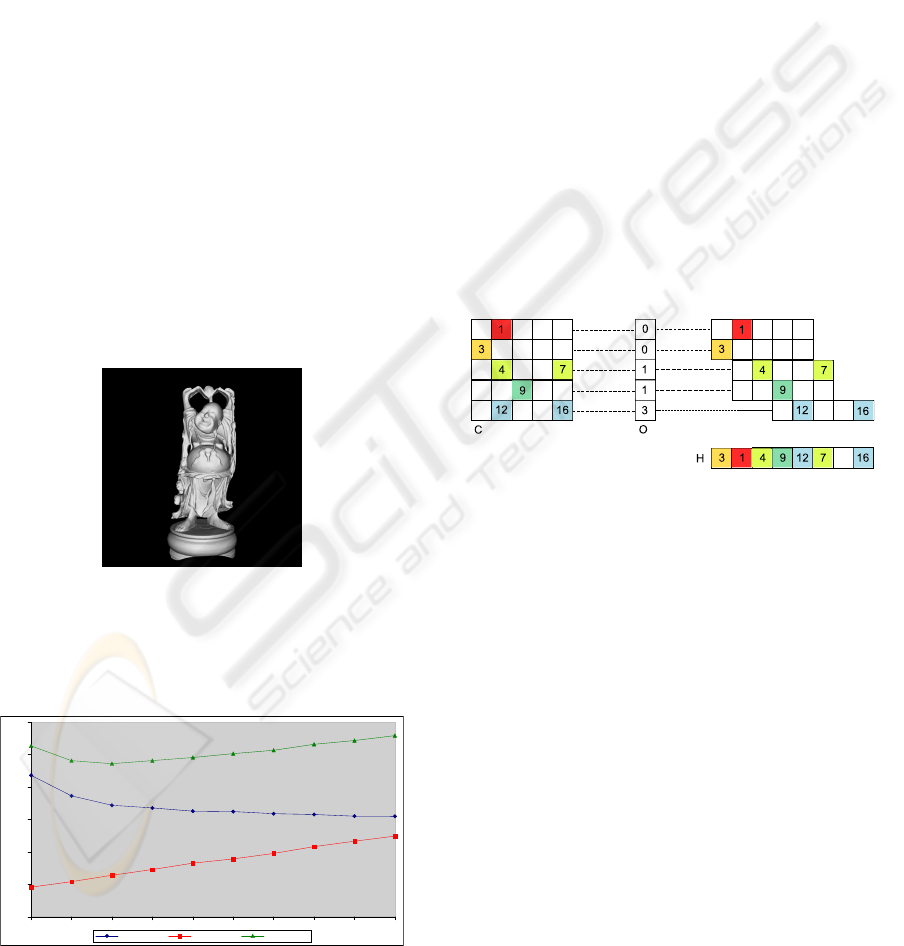
We empirically chose the grid density parameter

by analyzing the behavior for the Buddha scene (Fig-

ure 1) as can be seen in the chart at Figure 2.

Figure 1: Buddha scene at 1024 × 1024 resolution.

We selected a grid density ρ of 32 since it features

adequate render time without having a severe impact

on time to image.

8 16 24 32 40 48 56 64 72 80

0.2

0.4

0.6

0.8

1.2

seconds

Render Time Build Time Time to Image

Figure 2: Timings for the Buddha scene according to grid

density.

3.2 Hashed Grid Construction

An array with cell offsets is a linear representation of

a sparse 3D matrix. Given the data is static, a perfect

hash function, with no collisions, can be computed.

Hashing was done using row displacement compres-

sion (Lagae and Dutr

e, 2008) in order to avoid storing

empty array cells. A description of the algorithm is

provided here as a courtesy to the reader.

The data structure for the hashed grid implemen-

tation consists of four static arrays. Array L is a 1D

array of machine words which contains the indexes of

all cell items. Array H (hash table) is a linearized and

hashed 3D array of machine word indexes into L. The

item list size for a cell i is given by H[i]−H[i+1]. Ar-

ray O (offset table) is a linearized 2D array of machine

word indexes into H. O has M

× M

size. Finally, ar-

ray D (domain bits) is similar to array C (which stores

an index to the beginning of the item list for each

cell) but with one bit per cell. D has N size where

N = M

× M

. D stores if a given cell is not

empty. Elements in the hash table can be accessed in

constant time.

Figure 3: Row displacement compression. The 2D matrix

C is compressed into hash table H by displacing the rows,

and storing the offset of each row in offset table O.

Hashed grid data structure construction proceeds as

follows. First the scene’s bounding box is com-

puted. Then the grid heuristic, described in Sec-

tion 3.1, is used to determine the grid dimensions

× M

= N.

Array D is allocated with size N and its bits are

initialized to zero. For each item whose bounding box

intersects a given cell i, D[i] is set to one. After this

step, D[i] is an array containing which cells are not

empty. D cells can be indexed in 1D as D[d(x,y,z)]

where:

d(x,y, z) = ((M

× z) + y) × M

) + x

The offset table can now be ﬁlled. First O is allo-

cated with size M

× M

. A temporary bit array bH,

is allocated with a size of double the number of non

empty cells and its bits initialized to zero, to aid in its

construction. For each grid row (y, z) in O, the small-

est offset is found, starting from the last offset. If a

given D[d(0,y, z) .. d(M

− 1, y,z)] row’s bits collide

MULTI-LEVEL GRID STRATEGIES FOR RAY TRACING - Improving Render Time Performance for Row

Displacement Compressed Grids

221

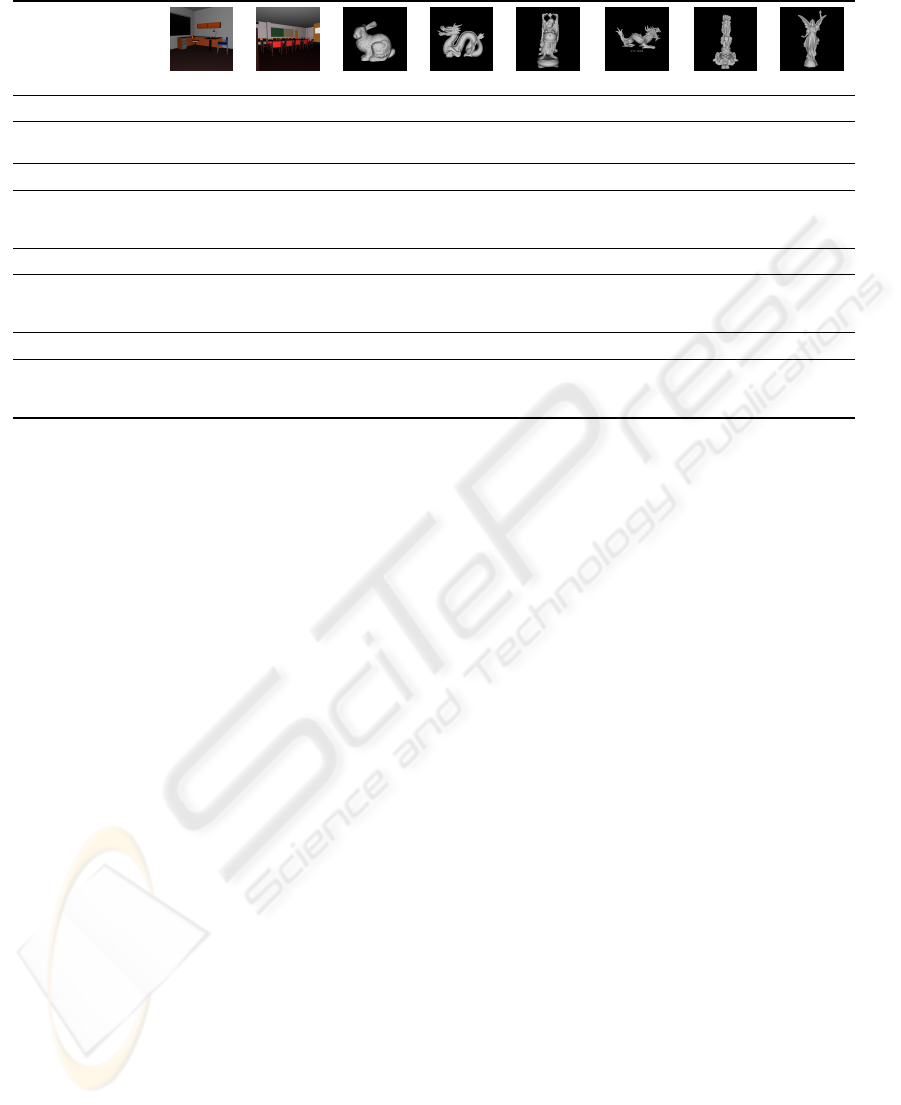
Table 1: Scene statistics and test results.

Ofﬁce Conference Bunny Dragon Buddha Asian Dragon Thai Statue Lucy

Scene

Triangles 36.31 K 282.76 K 69.45 K 871.41 K 1.09 M 7.22 M 10 M 28.06 M

Memory 910.05 KB 6.29 MB 1.21 MB 14.98 MB 18.67 MB 123.92 MB 171.66 MB 481.61 MB

Multi-Level Array Grid

Memory 7.06 MB 42.68 MB 17.62 MB 106.72 MB 109.36 MB 700.80 MB 0.99 GB -

Build Time 0.14 s 1.11 s 0.37 s 1.86 s 1.90 s 13.89 s 19.91 s -

Render Time 1.10 s 1.30 s 0.45 s 0.59 s 0.58 s 0.79 s 1.05 s -

One-Level Hashed Grid

Memory 552.59 KB 4.83 MB 0.98 MB 9.87 MB 12.68 MB 50.85 MB 78.75 MB 199.04 MB

Build Time 0.01 s 0.07 s 0.02 s 0.28 s 0.29 s 1.70 s 2.40 s 6.89 s

Render Time 2.01 s 2.13 s 0.56 s 0.75 s 0.66 s 1.42 s 1.60 s 1.61 s

Multi-Level Hashed Grid

Memory 1.55 MB 5.62 MB 2.39 MB 14.60 MB 15.59 MB 70.37 MB 105.78 MB 223.77 MB

Build Time 0.02 s 0.09 s 0.05 s 0.43 s 0.35 s 3.36 s 3.91 s 9.05 s

Render Time 1.87 s 2.04 s 0.49 s 0.42 s 0.40 s 0.75 s 0.78 s 0.94 s

with the bits in the current offset, at the temporary

bit array bH, then the offset is incremented and that

offset is tested for bit collisions.

Following this step, the offsets into the hash table

for each row (y,z) have been computed and stored into

O[o(y,z)] where:

o(y,z) = (M

× z) + y

The hash table can now be adequately computed.

First H is allocated with size NH equal to the position

of the last non empty bit in the temporary bit array bH

plus one and its machine words are initialized to zero.

The offsets into the item lists are then computed.

For each item whose bounding box intersects a

given cell i = (x,y, z), H[h(x,y,z)] is incremented by

one where:

h(x,y, z) = O[(M

× z) + y] + x

Note that the hash function h(x,y,z) will always

be valid in this case, since we are only inserting items

into cells which have already been determined to be

non empty in a prior step. At this point H stores how

many items are in each non empty cell.

The indexes of the item lists can now be com-

puted. However it is necessary, for the next step, to

know how many item indices have already been in-

serted during iteration of the item lists. For this it is

necessary to know, for each cell, the index into L for

the last item in that cells item list. The computation

for this step is done as follows:

for (i=1; i<=NH; ++i) {

H[i] += H[i-1];

}

At this point things should look pretty famil-

iar. Following this intermediate step, the sum of the

length of all item lists is stored at H[NH − 1]. Hence

L is now allocated with size H[NH − 1]. Items can

now be inserted into item list L, and each cell index

updated to point to the beginning of the item list. The

following procedure can be used:

for (i=NI-1; i>= 0; --i) {

// for each cell j intersected by object i

L[--H[j]] = i;

}

After this procedure is complete, L is ﬁlled with

all list item indexes, and each cell H[i] indexes into

the ﬁrst item of its item list in a linear fashion. All

indexes in the item list are sorted. This algorithm

has complexity linear in time to the number of scene

items, except for hash function computation, which

has worst case time complexity of O(M

4/3

) where M

is the number of cells in the grid.

3.3 Macrocells Construction

Next multi-level macrocells, as described in (Wald

et al., 2006), are built to skip empty cells in larger

steps during traversal. Macrocells overlay a coarser

grid over the ﬁnely divided grid. The macrocells for

each level consist of a 3D bit array with information

if a region of space is empty of not. To speed up this

construction step macrocells are downscaled by a fac-

tor of 6 on each extent. We arrived at this value by em-

pirically analyzing algorithm behavior for the tested

scenes. (Wald et al., 2006) reached the same value

with a different heuristic and test scenes. Macrocell

GRAPP 2010 - International Conference on Computer Graphics Theory and Applications

222

downscaling can be done with a quick 3D bitmap

scaling operation of 3D bitmap D.

There is no recursion during construction.

4 RESULTS AND DISCUSSION

In this section a comprehensive evaluation of the per-

formance of the grid rendering method described in

this paper is presented.

The methods implemented in this work were done

in C++ using the STL and Boost. Assembly code or

intrinsics were not used. All timings were done on a

computer with a single two-core 3GHz Intel Core 2

Duo CPU with 2GB of memory. Only a single thread

was employed. All images were rendered at a resolu-

tion of 1024×1024 with one ray per pixel and diffuse

shading.

Oﬃce Conference Bunny Dragon Buddha Asian Dragon Thai Statue Lucy

200

400

600

800

1000

1200

memory (MB)

Multi-Level Array Grid One-Level Hashed Grid Multi-Level Hashed Grid

Figure 4: Acceleration structure memory usage statistics

for the tested scenes.

Table 1 shows scene statistics such as number of

triangles, memory used by the triangles. Scene mem-

ory usage is computed by using 12 bytes per trian-

gle to store vertex index information (three machine

words for each vertex index), plus 12 bytes per ver-

tex (three ﬂoating point numbers for each coordinate).

This provides a two-fold decrease in memory used

for the tested scenes versus the scene storage method

used by (Lagae and Dutr

e, 2008). This was particu-

larly important given the system used for these tests

has much less memory than the system used by the

before mentioned authors. Ray-triangle intersection

was done using the (M

oller and Trumbore, 2005) in-

tersection algorithm because of its low memory re-

quirements.

The memory footprint for hashed grid implemen-

tations is roughly one order or magnitude lower than

for regular, non-compressed grids. Multi-level hashed

grids have slightly higher memory consumption than

one-level hashed grids as can be seen in Figure 4. In

particular the non-compressed multi-level array grid

algorithm exhausted available system memory for the

Lucy scene.

Oﬃce Conference Bunny Dragon Buddha Asian Dragon Thai Statue Lucy

build time (s)

Multi-Level Array Grid One-Level Hashed Grid Multi-Level Hashed Grid

Oﬃce Conference Bunny Dragon Buddha Asian Dragon Thai Statue Lucy

0.5

1.5

2.5

render time (s)

Multi-Level Array Grid One-Level Hashed Grid Multi-Level Hashed Grid

Figure 5: In the top chart, acceleration structure build time

statistics can be seen. At bottom, the chart has render time

statistics for the tested scenes. Timings are the average

of several test runs. Results for the proposed multi-level

hashed grid acceleration structure are at right.

The build time for hashed grids is short and

roughly linear with the number of triangles as can be

seen in Figure 5. This gives a short time to image

useful for dynamic scenes. Multi-level array grids be-

have poorly regarding build time, getting even worse

for the more complex scenes.

Render times, as expected, are better for the multi-

level grids. Multi-level hashed grids behave espe-

cially well for the larger tested scanned scenes, with

the most empty cells, having around twice the render-

time performance of one-level hashed grids due to

macrocells. These results are better than the 30%

speedup reported by (Wald et al., 2006). For small

non-uniform density scenes, such as Ofﬁce and Con-

ference, performance is better using the classic adap-

tive multi-level array grid scheme.

For comparison purposes (Lagae and Dutr

e, 2008)

report a build time of 1.76 s and a render time of 1.43

s for the Thai Statue scene at 1024 × 1024 resolu-

tion using the one-level hashed grid algorithm. The

implementation of that algorithm in our framework

has a build time of 2.40 s and a render time of 1.60

s for the same scene. Using the multi-level hashed

grid algorithm, described here, build time is 3.91 s

but render time is much improved at 0.94 s for the

same scene. This is a 52% render time performance

MULTI-LEVEL GRID STRATEGIES FOR RAY TRACING - Improving Render Time Performance for Row

Displacement Compressed Grids

223

improvement versus (Lagae and Dutr

e, 2008), even

using worse hardware.

Estimated algorithm performance is ≈ 4.26 FPS

for the Thai Statue scene at 1024×1024 resolution on

a quad core system assuming a linear speedup, com-

mon in ray tracing. This compares well with the 3.14

FPS KD-tree performance achieved by (Shevtsov

et al., 2007) on such a system.

5 CONCLUSIONS AND FUTURE

WORK

Multi-level hashed grids have good behavior for large

scanned models, having twice the render-time perfor-

mance of one-level hashed grids, with a small penalty

in terms of build time or memory usage. They suc-

cessfully combine the better traits of classic multi-

level array grids and one-level hashed grids, manag-

ing to provide best of class performance for scanned

scenes.

There still seems to be room for improvement

in regards to speeding up grid traversal by skipping

empty cells. Possibilities include proximity clouds

(Cohen and Sheffer, 1994) and macro-regions (Dev-

illers, 1989). This work also does not employ SIMD

instructions or ray coherence. All of these techniques

have a chance of signiﬁcantly improving performance

and should be worthy of further pursuit.

ACKNOWLEDGEMENTS

It would not have been possible to make the tests in

this work without the scanned models from the Stan-

ford 3D Scanning Repository. Ofﬁce and Confer-

ence scenes were created by Anat Grynberg and Greg

Ward.

We would also like to thank the anonymous re-

viewers, for their comments helped improve this

work.

Supported by the Portuguese Foundation for

Science and Technology project VIZIR (PTD-

C/EIA/66655/2006).

REFERENCES

Amanatides, J. and Woo, A. (1987). A fast voxel traversal

algorithm for ray tracing. In Eurographics ’87, pages

3–10.

Cleary, J. and Wyvill, G. (1988). Analysis of an algorithm

for fast ray tracing using uniform space subdivision.

The Visual Computer, 4(2):65–83.

Cohen, D. and Sheffer, Z. (1994). Proximity clouds - an ac-

celeration technique for 3D grid traversal. The Visual

Computer, 11(1):27–38.

Devillers, O. (1989). The macro-regions: an efﬁcient space

subdivision structure for ray tracing. In Eurographics

’89, pages 27–38.

Fujimoto, A., Tanaka, T., and Iwata, K. (1986). Arts: Ac-

celerated ray-tracing system. Computer Graphics and

Applications, IEEE, 6(4):16–26.

Havran, V., Sixta, F., and Databases, S. (1999). Comparison

of hierarchical grids. Ray Tracing News, 12(1):1–4.

Ize, T., Shirley, P., and Parker, S. (2007). Grid creation

strategies for efﬁcient ray tracing. In Interactive Ray

Tracing, 2007. RT’07. IEEE Symposium on, pages 27–

32.

Jevans, D. and Wyvill, B. (1989). Adaptive voxel subdivi-

sion for ray tracing. In Graphics Interface ’89, pages

164–172.

Kalojanov, J. and Slusallek, P. (2009). A parallel algorithm

for construction of uniform grids. In Proceedings of

the 1st ACM conference on High Performance Graph-

ics, pages 23–28. ACM.

Kim, T., Moon, B., Kim, D., and Yoon, S. (2009). RACB-

VHs: random-accessible compressed bounding vol-

ume hierarchies. In SIGGRAPH 2009: Talks, page 46.

ACM.

Lagae, A. and Dutr

e, P. (2008). Compact, fast and robust

grids for ray tracing. Computer Graphics Forum (Pro-

ceedings of the 19th Eurographics Symposium on Ren-

dering), 27(8).

oller, T. and Trumbore, B. (2005). Fast, minimum stor-

age ray/triangle intersection. In International Con-

ference on Computer Graphics and Interactive Tech-

niques. ACM Press New York, NY, USA.

Shevtsov, M., Soupikov, A., and Kapustin, A. (2007).

Highly parallel fast kd-tree construction for interactive

ray tracing of dynamic scenes. In Computer Graphics

Forum, volume 26, pages 395–404. Citeseer.

Wald, I., Ize, T., Kensler, A., Knoll, A., and Parker, S.

(2006). Ray tracing animated scenes using coher-

ent grid traversal. In International Conference on

Computer Graphics and Interactive Techniques, pages

485–493. ACM Press New York, NY, USA.

Woo, A. (1992). Ray tracing polygons using spatial subdi-

vision. In Proceedings of the conference on Graph-

ics interface ’92, pages 184–191, San Francisco, CA,

USA. Morgan Kaufmann Publishers Inc.

GRAPP 2010 - International Conference on Computer Graphics Theory and Applications

224