
FUZZY FREQUENCY RESPONSE FOR UNCERTAIN DYNAMIC
SYSTEMS
Carlos Cesar Teixeira Ferreira and Ginalber Luiz de Oliveira Serra
Federal Institute of Education, Science and Technology of Maranh˜ao (IFMA)
Av. Get´ulio Vargas, 04, Monte Castelo, 65025-001, S˜ao Lu´ıs, MA, Brazil
Keywords:
Takagi-Sugeno fuzzy control, Uncertain dynamic systems, Frequency response analysis.
Abstract:
This paper focuses on the Fuzzy Frequency Response: Definition and Analysis for Uncertain Dynamic Sys-
tems. In terms of transfer function, the uncertain dynamic system is partitioned into several linear sub-models
and it is organized into Takagi-Sugeno (TS) fuzzy structure. The main contribution of this approach is demon-
strated, from a Theorem, that fuzzy frequency response is a boundary in the magnitude and phase Bode plots.
Low and high frequency analysis of fuzzy dynamic model is obtained by varying the frequency ω from zero
to infinity.
1 INTRODUCTION
The design of control systems is currently driven by
a large number of requirements posed by increas-
ing competition, environmental requirements, energy
and material costs, the demand for robust and fault-
tolerant systems. These considerations introduce ex-
tra needs for effective process control techniques. In
this context, the analysis and synthesis of compen-
sators are completely related to each other. In the
analysis, the characteristics or dynamic behaviour of
the control system are determined. In the design,
the compensators are obtained to attend the desired
characteristics of the control system from certain per-
formance criteria. Generally, these criteria may in-
volve disturbance rejection, steady-state erros, tran-
sient response characteristics and sensitivity to pa-
rameter changes in the plant.
Test input signals is one way to analyse the dy-
namic behaviour of real world system. Many test sig-
nals are available, but a simple and useful signal is the
sinusoidal wave form because the system output with
a sinusoidal wave input is also a sinusoidal wave, but
with a different amplitude and phase for a given fre-
quency. This frequency response analysis describes
how a dynamic system responds to sinusoidal inputs
in a range of frequencies and has been widely used in
academy, industry and considered essential for robust
control theory (Serra and Ferreira, 2010).
The frequency response methods were devel-
oped during the period 1930 − 1940 by Harry
Nyquist (1889 − 1976) (Nyquist, 1932), Hendrik
Bode (1905 − 1982) (Bode, 1940), Nathaniel B.
Nichols (1914− 1997) (James et al., 1947) and many
others. Since, frequency response methods are among
the most useful techniques and available to analyse
and synthesise the compensators. In (Jr, 1973), the
U.S. Navy obtains frequency responses for aircraft
by applying sinusoidal inputs to the autopilots and
measuring the resulting position of the aircraft while
the aircraft is in flight. In (Lascu et al., 2009), four
current controllers for selective harmonic compensa-
tion in parallel Active Power Filters (APFs) have been
compared analytically in terms of frequency response
characteristics and maximum operational frequency.
Most real systems, such as circuit components (in-
ductor, resistor, operational amplifier, etc.) are often
formulated using differential/integral equations with
uncertain parameters (Kolev, 1993). The uncertain
about the systems arises from aging, temperature vari-
ations, etc. These variations do not follow any of
the known probability distributions and are most of-
ten quantified in terms of boundaries. The classical
methods of frequency response do not explore these
boundaries for uncertain dynamic systems. To over-
come this limitation, this paper proposes the defini-
tion of Fuzzy Frequency Response (FFR) and its ap-
plication for analysis of uncertain dynamic systems.
209
Cesar Teixeira Ferreira C. and Luiz de Oliveira Serra G. (2010).
FUZZY FREQUENCY RESPONSE FOR UNCERTAIN DYNAMIC SYSTEMS.
In Proceedings of the 7th International Conference on Informatics in Control, Automation and Robotics, pages 209-212
DOI: 10.5220/0002815402090212
Copyright
c
SciTePress
2 FORMULATION PROBLEM
This section presents some essentials concepts for the
formulation and development of this paper Fuzzy Fre-
quency Response for Uncertain Dynamic Systems.
2.1 Uncertain Dynamic Systems
In terms of transfer function, the general form of an
uncertain dynamic systems is given by Eq. 1, as de-
picted in Fig.1.
X
ν
ν
Y
G(s, )
Figure 1: TS fuzzy model.
G(s, ν) =
Y(s, ν)
X(s)
=
b
α
(ν)s
α
+ b
α−1
(ν)
α−1
+ . . . + b
α
(ν)s
α
+ b
1
(ν)s+ b
0
(ν)
s
β
+ a
β−1
(ν)s
β−1
+ . . . + a
1
(ν)s+ a
0
(ν)
(1)
where: X(s) and Y(s, ν) represents the input and the
output of uncertain dynamic systems; a
∗
(ν) and b
∗
(ν)
are the varying parameters; ν(t) is the time varying
scheduling variable; s is the Laplace operator; α and
β are the orders of the numerator and denominator of
the transfer function, respectively (with β ≥ α). The
scheduling variable ν belongs to a compact set ν ∈ V,
with its variation limited by |
˙
ν| ≤ d
max
, with d
max
≥ 0.
This formulation is very efficient and the fuzzy fre-
quency response of (1) can be used for stability anal-
ysis and robust control design.
2.2 Takagi-Sugeno Fuzzy Dynamic
Model
The inference system TS, originally proposed in (Tak-
agi and Sugeno, 1985), presents in the consequent a
dynamic functional expression of the linguistic vari-
ables of the antecedent. The i
[i=1,2,...,l]
-th rule, where
l is the rules numbers, is given by
Rule
(i)
:
IF ˜x
1
is F
i
{1,2,...,p
˜x
1
}|
˜x
1
AND. . . AND ˜x
n
is F
i
{1,2,...,p
˜x
n
}|
˜x
n
THEN y
i
= f
i
(˜x) (2)
where the total number of rules is l = p
˜x
1
× . . . ×
p
˜x
n
. The vector ˜x = [ ˜x
1
, . . . , ˜x
n
]
T
∈ ℜ
n
contain-
ing the linguistics variables of antecedent, where T
represents the operator for transpose matrix. Each
linguistic variable has its own discourse universe
U
˜x
1
, . . . , U
˜x
n
, partitioned by fuzzy sets representing
its linguistics terms, respectively. In i-th rule, the
variable ˜x
{1,2,...,n}
belongs to the fuzzy set F
i
{ ˜x
1
,..., ˜x
n
}
with a membership degree µ
i
F
{ ˜x
1
,..., ˜x
n
}
defined by a
membership function µ
i
{ ˜x
1
,..., ˜x
n
}
: ℜ → [0, 1], with
µ
i
F
{ ˜x
1
,..., ˜x
n
}
∈ {µ
i
F
1|{ ˜x
1
,..., ˜x
n
}
, µ
i
F
2|{ ˜x
1
,..., ˜x
n
}
, . . . , µ
i
F
p|{ ˜x
1
,..., ˜x
n
}
},
where p
{ ˜x
1
,..., ˜x
n
}
is the partitions number of the dis-
course universe associated with the linguistic vari-
able ˜x
1
, . . . , , ˜x
n
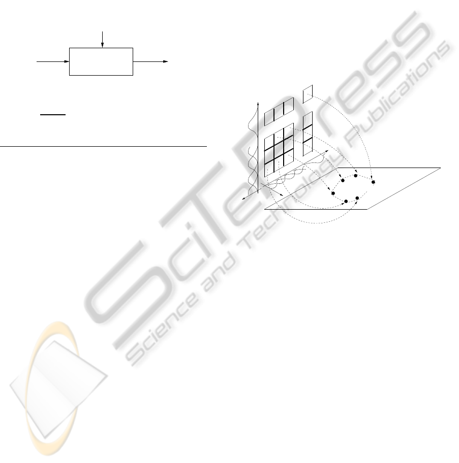
. The output of the TS fuzzy dynamic
model is a convex combination of the dynamic func-
tional expressions of consequent f
i
(˜x), without lost of
generality for the bidimensional case, as illustrated in
Fig. 2, given by Eq. 3.
...
1
F
| x 1
F
| x 1
F
| x 1
F
|
x 1
~
x
2
x
2
x
2
x
2
x
2
x2x 1,( )f1
x2x 1,( )2f
x2x 1,( )
x
2x 1,( )f4
x2x 1,( )f5
x2x 1,( )f3
Rule
Polytope
1 3 2 p
...
...
...
...
...
2
3
p
Consequent space
Rule
...
1
Antecedent space
F
|
~
F
|
F
|
F
|
fl
...
...
...
...
x
Figure 2: Fuzzy dynamic model: A TS model can be re-
garded as a mapping from the antecedent space to the space
of the consequent parameters one.
y(˜x, γ) =
l
∑
i=1
γ
i
(˜x) f
i
(˜x) (3)
where γ is the scheduling variable of the TS fuzzy dy-
namic model. It can be observed that the TS fuzzy
dynamic system, which represents any uncertain dy-
namic model, may be considered as a class of sys-
tems where γ
i
(˜x) denotes a decomposition of linguis-
tic variables [ ˜x
1
, . . . , ˜x
n
]
T
∈ ℜ
n
for a polytopic geo-
metric region in the consequent space from the func-
tional expressions f
i
(˜x).
3 FUZZY FREQUENCY
RESPONSE (FFR): DEFINITION
This section will present how a TS fuzzy model of
an uncertain dynamic system responds to sinusoidal
inputs, which in this paper is proposed as the defini-
tion of fuzzy frequency response. The response of a
TS fuzzy model to a sinusoidal input of frequency ω
1
ICINCO 2010 - 7th International Conference on Informatics in Control, Automation and Robotics
210

in both amplitude and phase, is given by the transfer
function evaluated at s = jω
1
, as illustrated in Fig. 3.
E(s)
l
i = 1
γ
i W (s)
i
Y(s)
Σ
Figure 3: TS fuzzy transfer function.
For this TS fuzzy model,
Y(s) =
"
l
∑
i=1
γ
i
W
i
(s)
#
E(s) (4)
Consider
l
∑
i=1
γ
i
W
i
( jω) a complex number for a
given ω, as
l
∑
i=1
γ
i
W
i
( jω) =
=
l
∑
i=1
γ
i
W
i
( jω)
e
jφ(ω)
=
l
∑
i=1
γ
i
W
i
( jω)
∠φ(ω) =
=
l
∑
i=1
γ
i
W
i
( jω)
∠arctan
"
l
∑
i=1
γ
i
W
i
( jω)
#
(5)
Then, for the case that the input signal e(t) is si-
nusoidal, that is,
e(t) = Asinω
1
t (6)
the output signal y
ss
(t), in the steady state, is given
by
y
ss
(t) = A
l
∑
i=1
γ
i
W
i
( jω)
sin[ω
1
t + φ(ω
1
)] (7)
As result of the fuzzy frequency response defini-
tion, it is proposed the following theorem:
Theorem 3.1. Fuzzy frequency response is a region
in the frequency domain, defined by the consequent
sub-models and from the operating region of the an-
tecedent space.
Proof. Considering that the parameter ν(t) is uncer-
tain and can be represented by linguistic terms, once
known its discurse universe, as shown in Fig. 4, the
activation degrees, h
i
(
˜
ν)|
i=1,2,...,l
, are also uncertain,
since it dependes of the dynamic system:
Membership degree
F
| }{
F
|
p
ν 1,..., ν n
~
1,...,
~
nν ν
1F
|
µ
}{ nν 1,..., ν
µ
}{
F
|
2
1,..., nνν
0
1
}{|
F3
}
− Discurse universe
}{ n}{
F
|
2
1,..., n1,..., n
n
~ ~
1, ... ,
ν 1,..., ννν
ν ν
ν ν
1 n
,...,ν∗ ν∗
{
µ
1,..., nν ν
U U
...
Fuzzy sets representing linguistics terms
1
Figure 4: Functional description of the linguistic variables:
linguistic terms, discurse universes and membership de-
grees.
h
i
(
˜
ν) = µ
i
F
˜
ν
∗
1
⋆ µ
i
F
˜
ν
∗
2
⋆ . . . ⋆ µ
i
F
˜
ν
∗
n
(8)
where
˜
ν
∗
{1,2,...,n}
∈ U
˜
ν
{1,2,...,n}
, respectively, and ⋆ is
a fuzzy logic operator.
So, the normalized activation degrees
γ
i
(ν)|
i=1,2,...,l
, are also uncertain, as shown in:
γ
i
(
˜
ν) =
h
i
(
˜
ν)
l
∑
r=1
h
r
(
˜
ν)
(9)
This normalization implies
l
∑
k=1
γ
i
(
˜
ν) = 1 (10)
The output of the TS fuzzy model is a weighted
sum of the consequent functional expression, e.g.,
a linear convex combination of the local functions
f
i
(
˜
ν), and is given by
y(
˜
ν) =
l
∑
i=1
γ
i
(
˜
ν) f
i
(
˜
ν) (11)
Let F(
˜
ν) a vectorial space of transfer functions
with degree ≤ l and f
1
(s), f
2
(s), . . . , f
l
(s) transfer
functions which belongs to this vectorial space. A
transfer function f(s) ∈ F(
˜
ν) must be a linear convex
combination of the vectors f
1
(s), f
2
(s), . . . , f
l
(s). So
f(s) = γ
1
f
1
(s) + γ
2
f
2
(s) + . . . + γ
l
f
l
(s) (12)
f(s) =
l
∑
i=1
γ
i
(
˜
ν) f
i
(
˜
ν) (13)
The TS fuzzy model must attend the polytope
property. So, the sum of the normalized activation
degree must be equal to 1, as shown in Eq (10). To
satisfy this property, each rule must be singly acti-
vated. This condition is called boundary condition. In
this way, the following results are obtained:
If just the rule 1 is activated, it has (γ
1
= 1, γ
2
=
0, γ
3
= 0, . . . , γ
l
= 0). Hence,
FUZZY FREQUENCY RESPONSE FOR UNCERTAIN DYNAMIC SYSTEMS
211

f(s) = 1f
1
(s) + 0f
2
(s) + . . . + 0 f
l
(s) = f
1
(s)
(14)
From (5), it has
f( jω) =
f
1
( jω)
∠ f
1
( jω) (15)
If just the rule 2 is activated, it has (γ
1
= 0, γ
2
=
1, γ
3
= 0, . . . , γ
l
= 0). Hence,
f(s) = 0f
1
(s) + 1f
2
(s) + . . . + 0 f
l
(s) = f
2
(s)
(16)
From (5), it has
f( jω) =
f
2
( jω)
∠ f
2
( jω) (17)
If just the rule l is activated, it has (γ
1
= 0, γ
2
=
0, γ
3
= 0, . . . , γ
l
= 1). Hence,
f(s) = 0f
1
(s) + 0f
2
(s) + . . . + 1 f
l
(s) = f
l
(s)
(18)
From (5), it has
f( jω) =
f
l
( jω)
∠ f
l
( jω) (19)
Note that
f
1
( jω)
∠ f
1
( jω) and
f
l
( jω)
∠ f
l
( jω) define a boundary region. Under
such circumstances, it seems plausible that the fuzzy
frequency response for uncertain dynamic systems
converges to a boundary in the frequency response,
as shown in Fig.5.
4 CONCLUSIONS
The Fuzzy Frequency Response: Definition and Anal-
ysis for Uncertain Dynamic Systems is proposed in
this paper. It was shown that the fuzzy frequency re-
sponse is a region in the frequency domain, defined
by the consequent linear sub-models G
i
(s), from op-
erating regions of the uncertain dynamic system, ac-
cording to the proposed Theorem 3.1. This formula-
tion is very efficient and can be used for robust stabil-
ity analysis and control design for uncertain dynamic
systems.
Upper limit
Lower limit
Polytope
1 3 2 p
...
...
...
...
...
2
3
p
Rule
...
1
Antecedent space
F
|
~
F
|
F
|
F
|
fl
...
...
...
...
...
Consequent space
MagnitudePhase
Frequency Response
Frequency
Frequency
Mapping
Rule
~
1
ν
F
| 1
ν
F
| 1
F
| 1
F
ν 1 | νν
2
2
2
2
ν
ν
ν
ν
2
ν
f1
f
( ) 1, 22
f3
( ) 1, 2
f4 ( ) 1, 2
ν 2 1, ν( )
ν ν
ν ν
ν ν
( ) 1, 2
f5 ( ) 1, 2
ν ν
ν ν
Upper limit
Lower limit
Figure 5: Fuzzy frequency response: mapping from the
consequent space to the region in the frequency domain.
ACKNOWLEDGEMENTS
The authors wish to express their gratitude for
FAPEMA and CAPES by support of this research.
REFERENCES
Bode, H. W. (1940). Feedback amplifier design. Bell Sys-
tems Technical Journal, 19:42.
James, H. M., Nichols, N. B., and Phillips, R. S. (1947).
Theory of servomechanisms. McGraw-Hill, MIT Ra-
diation Laboratory Series. New York.
Jr, A. P. S. (1973). Determination of aircraft response car-
acteristics in approach/landing configuration for mi-
crowave landing system program. In Report FT-61R-
73, Naval Air Test Center. Patuxent River, MD.
Kolev, L. V. (1993). Interval methodsfor circuit analysis.
Singapore: World Scienhfic.
Lascu, C., Asiminoaei, L., Boldea, I., and Blaabjerg, F.
(2009). Frequency response analysis of current con-
trollers for selective harmonic compensation in ac-
tive power filters. IEEE Transactions on Industrial
Eletronics, 56(2).
Nyquist, H. (1932). Regeneration theory. Bell Systems
Technical Journal.
Serra, G. L. O. and Ferreira, C. C. T. (2010). Fuzzy fre-
quncy response: Definition and analysis for nonlinear
dynamic systems. IEEE International Symposium on
Industrial Electronics.
Takagi, T. and Sugeno, M. (1985). Fuzzy identification of
systems and its applications to modeling and control.
IEEE Trans. Syst. Man. Cyber, 15:116–132.
ICINCO 2010 - 7th International Conference on Informatics in Control, Automation and Robotics
212
