TREE-STRUCTURED TEMPORAL INFORMATION FOR FAST

HISTOGRAM COMPUTATION

everine Dubuisson

Laboratoire d’Informatique de Paris 6 (LIP6/UPMC), 104 avenue du Pr

esident Kennedy, 75016, Paris, France

Keywords:

Fast histogram computation, Integral histogram.

Abstract:

In this paper we present a new method for fast histogram computing. Based on the known tree-representation

histogram of a region, also called reference histogram,, we want to compute the one of another region. The

idea consists in computing the spatial differences between these two regions and encode it to update the

histogram. We never need to store complete histograms, except the reference image one (as a preprocessing

step). We compare our approach with the well-known integral histogram, and obtain better results in terms of

processing time while reducing the memory footprint. We show theoretically and with experimental results

the superiority of our approach in many cases. Finally, we demonstrate the advantage of this method on a

visual tracking application using a particle ﬁlter by improving its time computing.

1 INTRODUCTION

Histograms are often used in image processing for

feature representation (colors, edges, etc.). The com-

plex nature of images implies a large amount of infor-

mation to be stored in histograms, requiring more and

more computation time. Many approaches in com-

puter vision require multiple retrievals of histograms

for rectangular patches of an input image. Each one

is developed for a speciﬁc application, such as for im-

age retrieval (Halawani and Burkhardt, 2005), con-

trast enhancing (Caselles et al., 1999) or object recog-

nition (Gevers, 2001). In such approaches, we dispose

a reference histogram and try to ﬁnd the region of the

current image whose histogram is the most similar.

The similarity is given by a measure that has to be

computed between each target histogram and the ref-

erence one. This implies the computation of a lot of

target histograms, that can be very time consuming,

and may also need a lot of storage. The main goal

is then to reduce the computation time, while using

small data structures, requiring less memory.

In this article, we propose a new histogram com-

putation by using a data structure only coding the

pixel differences between two frames of a video se-

quence. This data structure is updated over time on

pixel changes information and is used to deﬁne the

histogram of the whole new image or a part of it.

We never need to store the complete histogram and

our representation is compact because it only contains

variation information between two frames. The main

advantages of our approach are that it is not dependent

on the histogram quantization (i.e. number of bins),

it is fast to compute (comparing to other approaches)

and compact. Section 2 reviews some of the previ-

ous works on fast histogram computation. Section 3

presents our method compared with the well-known

integral histogram. Section 4 gives some theoreti-

cal considerations about time computation and size

of storage needed. In Section 5, some experimental

results show the beneﬁt of our approach. In Section 6

we illustrate the capability of our method on a real ap-

plication: object tracking using particle ﬁltering. Fi-

nally, we give concluding remarks in Section 7.

2 PREVIOUS WORKS

An histogram is computed into a region by brows-

ing all the pixels of this region. If lots of histograms

have to be computed locally around a set of salient

points, it can be advantageous to use the histogram

of a nearby region and to update it to obtain the his-

togram of the current region, instead of computing all

the histograms. This can be applied in cases of spa-

tial ﬁltering, but also in temporal ﬁltering in video se-

quences, when trying to ﬁnd displacements of objects

between frames. A lot of works have been proposed

to reduce the histogram computing time.

Dubuisson S. (2010).

TREE-STRUCTURED TEMPORAL INFORMATION FOR FAST HISTOGRAM COMPUTATION.

In Proceedings of the International Conference on Computer Vision Theory and Applications, pages 13-22

DOI: 10.5220/0002815800130022

 SciTePress

One of the ﬁrst work on redundancy computation re-

duction was proposed by (Tang et al., 1979), in the

context of image ﬁltering. Considering the histogram

of a region R, the histogram of a region Q is com-

puted by keeping the histogram of their intersection

region, removing the pixels of R that do not belong

to Q, and adding those from Q that do not belong to

R. This approach is efﬁcient only in cases of large

intersection between regions. Recently this method

has been improved by (Perreault and Hebert, 2007) in

the context of median ﬁltering. In (Sizintsev et al.,

2008) the authors present the distributive histogram.

They use the property for disjoint regions R and Q

that H(R

Q) = H(R) + H(Q). Their approach can

then easily be adapted to non-rectangular regions that

is not the case of previous approaches.

A fast way to compute histograms in terms of

time computation is the integral histogram (Porikli,

2005) (IH), inspired from integral images (Viola and

Jones, 2001), that is now used in many applica-

tions needing massive histogram computations by lo-

calized searches, especially in recent tracking algo-

rithms (Adam et al., 2006; Wang et al., 2007). This

approach is inspired from integral image and consists

in computing the histogram of any region of an im-

age using only four operations (two additions and two

subtractions). IH is a cumulative function whose cells

IH(r, c) contain the histogram of an image area con-

taining its r ﬁrst rows and c ﬁrst columns. Then:

IH(r, c) = I(r, c) + IH(r − 1, c)

+ IH(r, c − 1) − IH(r − 1, c − 1)

Once the integral histogram has been computed

over all cells, we can derive any histogram of a

sub-region only using four elementary operations,

see (Porikli, 2005) for more details. For example, the

histogram of a w × h region R with pixel (r,c) as bot-

tom right corner is given by:

= IH(r, c) − IH(r − h, c)

− IH(r, c −w) + IH(r − h, c − w)

The main drawback of integral histogram is the large

amount of data needed to be stored. For an N × M

image, the size of the array IH needed is N × M × B,

where B is the number of bins in the histogram. We

can ﬁnd a good comparative study of some of these

previous exposed method in (Sizintsev et al., 2008).

However, our approach is totally different than previ-

ous ones: we never need to encode histograms (except

the reference one), but only the temporal differences

between two images, and use them to determine new

histograms. The size of the data structure, and the his-

togram computation time only depends on the varia-

tions between frames.

3 PROPOSED APPROACH:

TEMPORAL HISTOGRAM

Assume that we have a reference histogram H (from

the reference image I

), and want to compute his-

tograms in a new image I

only using H and temporal

variations between I

and I

. Temporal variations are

obtained with the image difference and encoded by a

tree data structure with height h

= 3. Nodes at the

level h = 1 correspond to the rows r

of the image I

where there is a difference with I

, and nodes at the

level h = 2 correspond to the columns numbers c

Leaf nodes contain, for each pixel (r

, c

), the differ-

ence between I

and I

, the initial bin it was belonging

to in H, and the bin it will belong to in the histogram

of the updated histogram. Figure 1 shows a basic ex-

ample of the construction of this data structure. On

the left, the image difference between I

and I

shows

only four different pixels, situated in three different

rows r

, r

and r

, and four different columns c

, c

and c

. For each pixel (r, c), we also have to store

its original and new bins, respectively b

and b

. Al-

gorithm 1 summarizes this process.

Algorithm 1. Temporal data structure construction.

T ← {}

Compute the image difference D = I

− I

for all D(r, c) 6= 0 do

← bin of I

(r, c); b

← bin of I

(r, c)

if node r does not exist in T then

Create branch r − c − (b

) in T

else

Add branch c − (b

) to node r in T

end if

end for

Figure 1: Construction of the data structure associated with

the image reference I

, on the left. For each non-zero value

pixel of I

, we store its new row number r

, column number

and original and ﬁnal bins, respectively b

and b

Once we have the reference histogram H

and the dif-

ference tree T , we can derive any histogram of a re-

VISAPP 2010 - International Conference on Computer Vision Theory and Applications

gion R in I

, as described in Algorithm 2. We then

just need to browse the data structure to determine if

some pixels have changed in this region between the

two images. For each changed pixel, we have to mod-

ify H

by removing one from the bin b

and adding

one to the bin b

. This is a very simple but efﬁcient

way to compute histograms because we just perform

the necessary operations (where change has been de-

tected). In the next Section, we give some theoretical

comparative results between our approach and inte-

gral histogram.

Algorithm 2. Histogram computation of a region R.

Extract the sub-tree T

from T , containing chang-

ing pixels in R between the two frames

for all node branch r − c − b

− b

in T

) ← H

) − 1

) ← H

) + 1

end for

4 THEORETICAL STUDY:

MEMORY AND

COMPUTATION COST

IH is, in our opinion, the best in the sense that it re-

quires low computation time and is ﬂexible enough

to adapt to many applications therefore it is the one

we have chosen for comparison with our approach.

In this section, we the compare our approach with IH

in terms of number of operations necessary to com-

pute histograms, and size of storage needed for the

data structures. We are considering an image I of size

N × M, and B is the number of bins in the histograms.

The histogram of the reference image has to be com-

puted as a preliminary step for both approaches: we

then do not consider this common step. We also do

not consider the allocation operations for the two data

structures (an array for IH and a tree for TH), but this

is clear that the tree needs less allocation operations

than an array, for a ﬁxed number of pixels, because

it only stores 4 values per changing pixel, whereas IH

stores a whole histogram per pixel. The determination

of the bin of a current pixel requires one division and

one ﬂoor: we call f

this operation, and a an addition

(or a subtraction). Both methods require two steps:

1. the data structure construction, then

2. the data access for the computation a a new his-

togram.

We ﬁrst consider and compare independently both

steps.

4.1 Construction of Data Structures

For IH, we need to browse all pixels I(r,c) of the im-

age, determine its bin value, and compute the integral

histogram using four operations a (see Section 2), for

each bin of the histogram. This part then needs a total

number of operations of:

)

= (4a + f

)NMB

This number of operations is a constant.

For TH, we ﬁrst need to ﬁnd non-zero values in the

image difference D (NMa operations). By scanning

D in the lexicographic order, we then create a branch

in the tree data structure for each non-zero value: let’s

be s the total number of non-zero value pixels (s ≤

(N × M)). For each of the s changing pixel, we have

to determine its new bin. The number of operations

needed for the construction of the tree is then:

)

= s f

+ NMa

Thus, to compare with IH, we have to consider two

special cases:

• In the best case, all the pixels in the image dif-

ference are zero-valued pixels: we need (n

)

NMa operations to construct T.

• In the worst case, all the pixel values of the image

difference are different from zero, the construc-

tion of T can be done using a total number of op-

erations of:

)

= NM f

+ NMa = NM(a + f

)

Even in the worst case (all pixels have changed), the

number of operations necessary for the construction

of T is less than the one necessary for the integral

histogram construction. It should also be noticed that

)

does not depend on the number B of bins of

the histogram because we do not encode histogram

(and so do not need to browse all bins), only temporal

changes between images.

4.2 Histogram Computations

For both approaches, we consider the problem of

computing the histogram H

of any region R = [R

] of a new image I

knowing histograms in I

. For

both approaches, we consider the data access or ex-

traction as a negligible constant respectively c

and

(experimental results in Section 5 show that this

is a not a strong assumption).

For IH we just need two additions and two subtrac-

tions between values stored in the data structure, for

each bin of the histogram (see Section 2). Then, to

TREE-STRUCTURED TEMPORAL INFORMATION FOR FAST HISTOGRAM COMPUTATION

compute any histogram, we need a constant number

of operations:

)

= 4aB

This is a bit more complicated for TH. We ﬁrst need

to extract the region R from T , if it does exist (we

have its histogram, see the introduction of this sec-

tion). Then, for each of the s

differences (s

≤ s if

R is a subregion of I, otherwise s

= s), we have to

remove one from the bin b

and add one to the bin b

The computation of a new histogram H

is done by a

total number of operations of:

)

= 2as

We consider the following special cases :

• In the best case, there is no difference between

the two considered regions: we need (n

)

= 0

operation.

• In the worst case, all the pixel values have

changed between the two regions, we can com-

pute the histogram using a number of operations

of:

)

= 2a|R|

where |R| = R

× R

is the number of pixels in R.

If R = I

, then (n

)

= 2aNM.

The efﬁciency of our approach for the new histogram

computation depends on the size of R and on the num-

ber of changing pixels between I

and I

. In the gen-

eral case, we have:

)

< (n

)

if 2as

< 4aB ⇔ s

< 2B

We then conclude that TH is better as long as the num-

ber of changing pixels is less than twice the number

of bins on the histogram.

4.3 Total Computation

The total histogram computation time of a region in

the new image I

is ﬁxed for IH:

)

= (4a + f

)NMB + 4aB

For TH, it depends on two major factors: (i) the

number s of changing pixels between I

and I

and

the number s

of changing pixels between (R)

and

(R)

. We need a total number of operation:

)

= s f

+ NMa + 2as

As previously, we can distinguish two cases:

• In he best case, there is no differences between the

considered regions and then T is empty, we need:

)

= NMa operations.

• In the worst case, all the pixel are different be-

tween I

and I

, so they are between (R)

and

(R)

), and we then need at total number of op-

erations:

)

= NM(a + f

) + 2a|R|

If R = I

, (n

)

= NM(a + f

) + 2aNM =

NM(3a + f

We can compare the worst case with the ﬁxed number

)

. IH depends on the size N × M of the image

and on the number B of bins of the histogram. TH

depends on the size of the image (conditioning the

potential number of changing pixels s) but also on the

region on which we compute the histogram. But the

data structure construction step requires less opera-

tions for TH (see Section 4.1). An histogram compu-

tation will require a number of operation depending

on the number of changing pixels between I

and I

(see Section 4.2)

4.4 Storage

We now compare the quantity of information neces-

sary for both approaches.

For IH, we need a constant-size array, containing a

total number of cells of:

(c)

= NMB

We need one B-size array for each pixel (r, c),

corresponding to the histogram of the region from

rows 1 to N and columns 1 to M.

For TH we use a tree T as data structure whose size

depends on the number s of changing pixels between

images I

and I

. If we call n

the number of rows in

containing changing pixels, the number of nodes of

T is:

(c)

= n

+ 3s

i.e. n

for the rows, and 3 nodes for each changing

pixel. We can distinguish two cases :

• In the best case, there is no difference between

regions, T is empty: (c)

= 0.

• In the worst case, all the pixels are different, and

the size if the required data structure T is:

(c)

= N + 3NM

Then, in the worst case (i.e. all the pixels have

changed between the two images or regions, that can

rarely happen):

(c)

< (c)

if NMB < N(1 + 3M) ⇔ B ≤ 3

In the most common case, (c)

< (c)

if NMB <

+ 3s. It is more than probable that the number of

VISAPP 2010 - International Conference on Computer Vision Theory and Applications

changing pixels between the two images is less than

the total number of pixels. At most, if all these chang-

ing pixels are located on different rows (negative sce-

nario), we have n

+ 3s = s + 3s = 4s, so:

(c)

< (c)

if NMB < 4s ⇔ s >

NMB

Globally our histogram computation needs then less

storage.

The theoretical considerations about the number of

operations and storage needed for both approaches

developed in this section will next be veriﬁed with a

number of experimental results in the next Section.

5 EXPERIMENTAL RESULTS

In this section, we systematically compare integral

histogram (IH) with the proposed temporal histogram

(TH), since no method has been proved to be more

interesting than IH in terms of both computation time

and storage: it would not be relevant to perform com-

parisons with other methods based on this criteria.

In the next subsections, we call computation of a

histogram the two-steps process needed for both ap-

proaches: data structure construction and histogram

computation. All computation times reported in this

section correspond to the mean value over 100 differ-

ent tests.

5.1 Computation Time

In this section we propose to compare the computa-

tion times of integral and temporal histograms. In

Section 4, we have highlighted some parameters that

we directly involved, such as the number B of bins

of the histograms, the size N × M of the images, the

number s of changing pixels in the whole image, and

the number s

of changing pixels in the considered

region for histogram computation.

5.1.1 Video Sequences

Tests on different complete video sequences have

been performed. In this section we only present those

made on sequences “Walking” (15 frames of size

275 × 320), “Tennis” (89 frames of size 240 × 342)

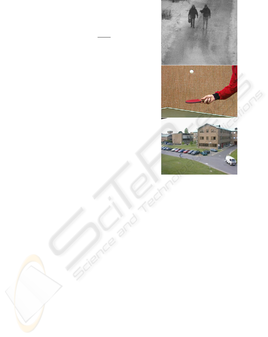
and “Parking” (231 frames of size 576 × 768), see ex-

amples of frames in Figure 2. Some frames of these

sequences are shown in Figure 3. In these tests, we

are interested in the total computation time (along all

the sequence) needed for the computation of the his-

togram of randomly chosen regions of size 10 × 10

in each I

(t > 1) depending on the number of bins.

Figure 2: A frame from, from top to bottom: “Walking”,

“Tennis” and “Parking” sequences.

We can see in Figure 3 that the computation times ob-

tained with our approach are lower for each one of

these sequences. This is in part due to the fact that

the computation of the array of the integral histogram

takes a lot of time (and is performed at each frame),

even if the histogram time computation (just requiring

four operations) is small. This also shows that our ap-

proach is relatively stable with respect to the increas-

ing number of bins B, contrary to integral histogram,

whose computation time increases with B (drastically

for B = 256). This is due to the fact that, contrary to

the IH, the number B of bins does not affect a lot the

computation time (see Section 4.3) of TH is there are

only few changing between two frames. As there is

no ”best” number of bins, and different bin numbers

can reveal different features of the data: it is difﬁ-

cult to determine an optimal number of bins, without

making strong assumptions about the shape of the dis-

tributions. With our approach, it is not necessary to

make such assumptions.

5.1.2 Image and Size Variations

The performance of our approach principally depends

on the number s of changing pixels. The larger s, the

more consuming the method is. We then have tested

TREE-STRUCTURED TEMPORAL INFORMATION FOR FAST HISTOGRAM COMPUTATION

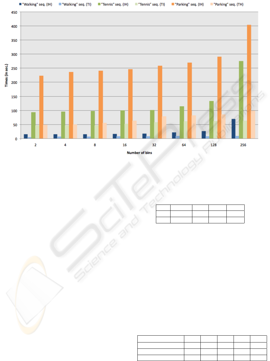
Figure 3: Tests on different video sequences (left column for an example of frame of, from top to bottom “Walking”, “Tennis”

and Parking” sequences). Bar diagram of an histogram computation time for both approaches, for different sequences and

increasing number of bins: “Walking” in blue, “Tennis” in green and “Parking” in orange (IH is represented as plain color,

TH as a transparency color).

the computation time as a function of s and compared

results with those obtained by the IH method.

In the ﬁrst test, on the “Walking” video sequence,

is used as reference image and we evaluated the

histogram computation time for a region in the next

frame. Tests have been performed in frames I

, I

and

, in which respectively 0%, 25% and 40% of the

pixels vary from the ﬁrst frame. Results are shown in

Figure 4, for different values of B. We can see that

the computation time of our approach increases as the

number of changing pixels increases, as highlighted

in Section 4 , but stay below the one obtained with

IH.

For the second test we have generated synthetic N ×N

images for different values of N and compared times

for the computation of the histogram with B = 16 bins

of this whole image (no pixel variation) for both ap-

proaches. Comparative results (in seconds) are re-

ported in Table 1. The increase of N does not inﬂu-

ence a lot our approach, much while drastically de-

creasing IH performance. As no pixel have changed

between the two considered frames, the small time

computation increasing for TH is just due to the pixel

scanning of the new image that takes more time for a

large image than a smaller one: this explains why the

time computation for TH is equal to 0.0064 seconds

for N = 256 and to 0.4 for N = 2048.

Table 1: Time computation (in sec.) of an histogram with

B = 16 bins depending on the size of the image.

N 256 512 1024 2048

IH 0.8 3.23 12.9 52.1

TH 0.0064 0.02 0.09 0.4

The third test consists in considering a 1024 ×

1024 synthetic image and simulating a number s of

changing pixels, then computing the histogram with

B = 16 bins of this new image. We have compared

the computation times between both approaches: re-

sults are reported in Table 2. The computation time

with our approach stays below IH’s one until s = 10

This is not surprising, because our approach depends

on the number of changing pixels between images.

Anyway, s should has to have a large value before in-

creasing drastically our computation time.

Table 2: Time computation (in sec.) of a histogram with

B = 16 bins of a 1024 × 1024 synthetic image after having

s changed pixels.

s 10

% changing pixels 0.01 0.1 1 10 100

IH 12.9 13 12.9 13.1 12.9

TH 0.14 0.24 0.47 2.49 27.6

VISAPP 2010 - International Conference on Computer Vision Theory and Applications

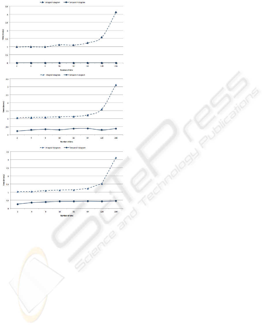
Figure 4: Comparison of integral histogram (IH) and tem-

poral histogram (TH) depending on the number of chang-

ing pixels between frames (“Walking” sequence, 275 × 320

frames). From top to bottom: 0% (between I

and I

), 25%

(between I

and I

) and 40% (between I

and I

) changing

pixels.

5.1.3 Number of Histogram Computations

The most time consuming part of IH is the construc-

tion of the array. However this array allows comput-

ing very quickly any histogram (or set of histograms)

using only four operations per histogram. In this sub-

section, we have launched a massive number of his-

togram computations and compared both approaches

in terms of computation time. The idea is to simu-

late the computation of target histograms in a search

window around a precise position, such as in spatial

ﬁltering or temporal ﬁltering (particle ﬁltering for ex-

ample). Test have been made on the “Walking” se-

quence. We have chosen to present the results for dif-

ferent values of B. Results are shown in Figure 5.

Once again the performance depends on the quan-

tization of the histograms. For a strong quantiza-

tion (B = 2 or 4), IH and TH become equivalent for

1000 computations of histograms. For B = 8,16, 32,

methods are equivalent for 5000 computations. For

B = 128, 10000 computations are needed, and 25000

for B = 256. This interesting result shows that we

can keep good results (compared to IH) with no need

for a strong quantization of the histogram: TH does

not need to approximate histograms to provide good

computation times, which is a real advantage for his-

togram based search applications. We can however

see one limitation of the proposed approach when

dealing with too much histograms. In Section 4.2

we mentioned that TH is better then IH as long as

the number of changing pixels is less than twice the

number of bins on the histogram. It is clear that the

performances of TH then is depends on the number

of changing pixels between the two considerer re-

gions on which we compute histograms, and that is

the reason why our computation times increase with

the number of computed histograms considered. We

can notice than for a small histogram quantization, we

give very good results. Our TH is the suitable for

visual tracking applications where it is better not to

quantify histograms too much.

5.2 Storage

In this section we show that our approach does not

need to store a lot of information, contrary to integral

histogram. Table 3 reports the size (number of ele-

ments) required for the two data structures used for

the test shown in Figure 4, middle row (between two

consecutive frames of the sequence). The number of

elements necessary for IH increases with the num-

ber of bins, according to the results of Section 4.4,

in which we found (c)

= NMB. For TH, it depends

on the number of changing pixels between the two

frames, (c)

= n

+ 3s. A pixel is said to be chang-

ing between the two images if he changes its bins

in the histogram. This notion then strongly depends

on the histogram quantization: the more histogram is

quantiﬁed, the less a pixel changes its bins between

two images. That is the reason why the number of

elements of our data structure indirectly depends on

B. Note that the number of elements needed for IH

does not change if images are really different, which

is not the case for TH. We report in Table 4 the size

of these data structures depending on the number s

of changing pixels between two images generated as

random 1024 × 1024 matrices (same experiments as

in Section 5.1.2). We ﬁx B = 16. For this case, the

number of elements necessary for integral histogram

TREE-STRUCTURED TEMPORAL INFORMATION FOR FAST HISTOGRAM COMPUTATION

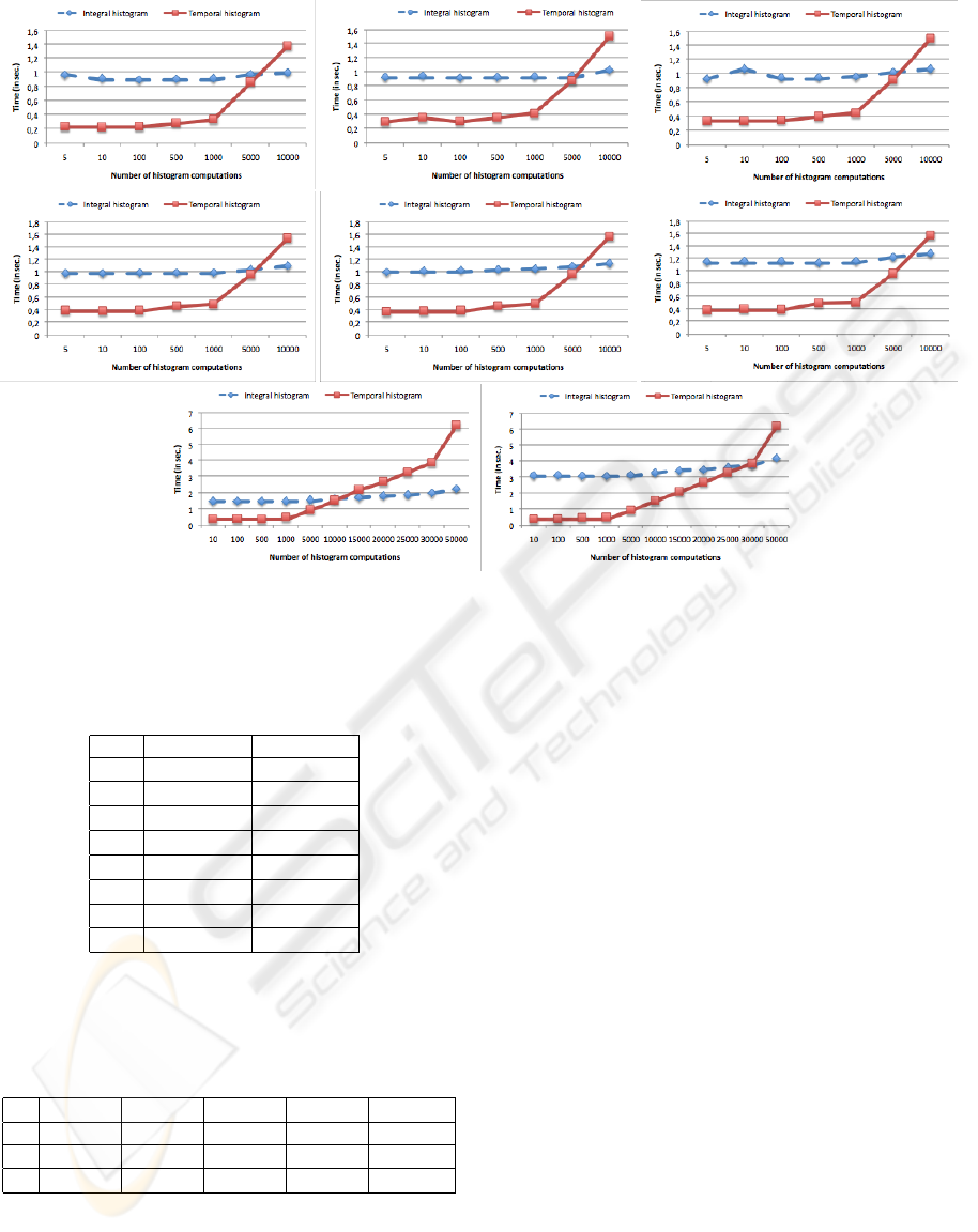
Figure 5: Comparison of IH (dotted lines) and TH (plain lines) results for a massive number of histogram computations, for

different values of B, from top to bottom, from left to right, 2, 4, 8, 16, 32, 64, 128 and 256.

Table 3: Size (number of elements) of data structures re-

quired for both approaches, depending on B, the test corre-

sponds to the one of the middle row of Figure 4.

B IH TH

2 1.76 × 10

9.1 × 10

4 3.52 × 10

1.78 × 10

8 7.04 × 10

2.93 × 10

16 1.4 × 10

4.5 × 10

32 2.81 × 10

4.5 × 10

64 5.63 × 10

4.5 × 10

128 1.12 × 10

4.53 × 10

256 2.25 × 10

4.53 × 10

Table 4: Size (number of elements) of data structures re-

quired for both approaches, depending on the number s of

changing pixels between two images generated ss random

1024 × 1024 matrix, for B = 16. Percentage (%) of chang-

ing pixel are reported on the second line of this table.

s 10

% 0.01 0.1 1 10 100

IH 1.6 × 10

1.6 × 10

TH 1.3 × 10

3.8 × 10

2.9 × 10

2.8 × 10

is ﬁxed such that (c)

= NMB = 1024 × 1024×16 =

1.6 × 10

. Even considering 10

changing pixels (i.e.

100% of the initial image) in the region the histogram

is computed, the number of elements needed to store

it is always below the one IH needs.

To our opinion, TH is a good alternative to his-

togram computation in a lot of cases because it gives

a compact description of temporal change and good

computation time results for histogram computation.

Moreover, we never need to store histograms (except

for the reference image), that is a real advantage when

working on video sequences (for these cases, the ref-

erence image is the ﬁrst of the sequence, and the his-

togram computation can be seen as a preprocessing

step).

6 INTEGRATION INTO

PARTICLE FILTER: FAST

PARTICLE WEIGHT

COMPUTATION

A good tracker should be able to predict in which

area of a new frame the object is. Among all the

methods, one can cite probabilistic trackers. In such

approaches, an object is characterized by a state se-

quence {x

}

k=1,...,n

whose evolution is speciﬁed by a

dynamic equation

= f

k−1

, v

)

The goal of tracking is to estimate x

given a set of ob-

servations. The observations {y

}

k=1,...,m

, with m < n,

VISAPP 2010 - International Conference on Computer Vision Theory and Applications

are related to the states by

= h

, n

)

Usually, f

and h

are vector-valued, nonlinear and

time-varying transition functions, and v

and n

are

white Gaussian noise sequences, independent and

identically distributed. Tracking methods based on

particle ﬁlters (Gordon et al., 1993; Isard and Blake,

1998) can be applied under very weak hypotheses and

consist of two main steps:

1. a prediction of the object states in the scene (us-

ing previous information), that consists in propa-

gating particles according to a proposal function

(see (Chen, 2003)) ;

2. a correction of this prediction (using an available

observation of the scene), that consists in weight-

ing propagated particles according to a likelihood

function.

Joint Probability Data Association Filter

(JPDAF) (Vermaak et al., 2004) provides an op-

timal data solution in the Bayesian framework ﬁlter

and uses a weighted sum of all measurements near

the predicted state, each weight corresponding to the

posteriori probability for a measurement to come

from an object. Between two observations, the set of

particles evolves according to an underlying Markov

chain, following a speciﬁc transition function. Given

a new observation, each particle is assigned a weight

proportional to its likelihood of belonging to a tracked

object. New particles are randomly sampled to favor

particles with higher likelihood. A classical approach

consists in integrating the color distributions given by

histograms into particle ﬁltering (P

erez et al., 2002),

by assigning a region (e.g. validation region) around

each particle and measuring the distance between the

distribution of pixels in this region and the one in the

area surrounding the object detected in a previous

frame. This context is ideal to test and compare our

approach in a speciﬁc framework.

For this test we measure the total computation

time of processing particle ﬁltering in the ﬁrst 60

frames of the “Rugby” sequence (240 × 320 frames,

see a frame in Figure 6): we are just interested on the

B = 16 bin histogram computation time around each

particle locations (that is the point of our paper). In

the ﬁrst frame of the sequence, the validation region

(ﬁxed size 30 × 40 pixels) containing the object to

track (one rugby player) is manually detected. JPADF

is then used along the sequence to automatically track

the object using N

particles. Then, the total computa-

tion times needed for each method is detailed below:

• For IH: one integral histogram H

in each frame

i = 1, . . . ,t of the sequence, then N

histogram

(one for each particle) computation using four op-

erations on H

• For TH: one integral histogram H (only in the ﬁrst

frame), one tree T

construction in each frame i =

1, . . . ,t of the sequence, then, a histogram update

for each particle using H and T

Computation times are reported in Table 5 for differ-

ent values of N

. Computation times are lower with

our approach until N

= 5000 (tests have shown that

for N

= 8500, computation times are the same for

both methods). Note that, in practice, we do not need

so much particles in a classical problem. Our ap-

proach permits real-time particle ﬁlter based tracking

for a reasonable number of particles, which is a real

advantage. Note that the purpose of this test was not

to deal with tracking performances (that is the reason

why we do not give any results about quality results):

we just want to show that integrating TH into particle

ﬁlter correction step instead of IH can accelerate the

process. Moreover, we have shown than for similar

computation times, we can use more particles into the

frameworks integrating TH. As it is well-known (Gor-

don et al., 1993) that the particle ﬁlter converges with

a high number of particles N

, we can argue that in-

tegrating TI into a particle algorithm improves visual

tracking quality. Note that we have obtained same

kinds of results on different video sequences (people

tracking on “Parking” sequence and ball tracking on

“Tennis” sequence”)

Table 5: Total computation times (in sec.) for all histograms

(B=16) in the particle ﬁlter framework, depending on the

number N

of particles.

50 100 1000 5000 10000

IH 47.75 47.4 47.5 50.48 53.59

TH 23.5 23.6 28.31 40.4 76.24

7 CONCLUSIONS

We have presented in this paper a new method for fast

histogram computation, called temporal histogram

(TH). The principle consists in never encoding his-

tograms, but rather temporal changes between frames,

in order to update a ﬁrst preprocessed histogram. This

technique presents two main advantages: we do not

need a large amount of information to store whole his-

tograms and it is less time consuming for histogram

computation. We have shown by theoretical and ex-

perimental results that our approach outperforms the

well-known integral histogram in terms of total com-

putation time and quantity of information to store.

Moreover, the introduction of TH into the particle ﬁl-

tering framework has shown its usefulness for real-

TREE-STRUCTURED TEMPORAL INFORMATION FOR FAST HISTOGRAM COMPUTATION

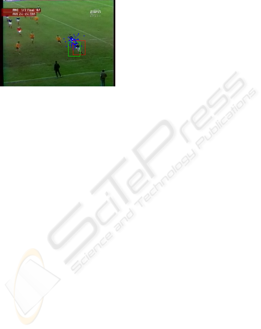
Figure 6: Example frame of the “Rugby” sequence: red

rectangle is the validation region, green one the target re-

gion associated to one particle. Blue crosses symbolize

particle positions in frame around which we compute histi-

grams.

time applications in most common cases. Integral his-

togram requires the computation of the accumulator

array in each new image which takes a lot of time

(rarely taken into account in classical approaches).

TH computes histogram only if necessary (i.e. some

changes between images have been detected). Future

works will concern the generalization of this reason-

ing on different distance computation between his-

tograms, that requires to work directly on histogram

bins (Bhattacharyya (Bhattacharyya, 1943), L

norm,

euclidean distance etc.): the update would be done on

this distance, not on the histogram.

REFERENCES

Adam, A., Rivlin, E., and Shimshoni, I. (2006). Ro-

bust fragments-based tracking using the integral his-

togram. In Proc. IEEE Conf. on Computer Vision and

Pattern Recognition, pages 798–805.

Bhattacharyya, A. (1943). On a measure of divergence be-

tween two statistical populations deﬁned by probabil-

ity distributions. Bulletin of the Calcutta Mathemati-

cal Society, 35:99–110.

Caselles, V., Lisani, J., Morel, J., and Sapiro, G. (1999).

Shape preserving local histogram modiﬁcation. IEEE

Trans. on Image Processing, 8(2):220–230.

Chen, Z. (2003). Bayesian ﬁltering: From kalman ﬁlters to

particle ﬁlters, and beyond. Technical report, McMas-

ter University.

Gevers, T. (2001). Robust histogram construction from

color invariants. IEEE Transactions on Pattern Anal-

ysis and Machine Intelligence, 26:113–118.

Gordon, N. J., Salmond, D. J., and Smith, A. F. M. (1993).

Novel approach to nonlinear/non-gaussian bayesian

state estimation. Radar and Signal Processing, IEE

Proceedings F, 140(2):107–113.

Halawani, A. and Burkhardt, H. (2005). On using his-

tograms of local invariant features for image retrieval.

In IAPR Conference on Machine Vision Applications,

pages 538–541.

Isard, M. and Blake, A. (1998). Condensation - conditional

density propagation for visual tracking. International

Journal of Computer Vision, 29:5–28.

erez, P., Hue, C., Vermaak, J., and Gangnet, M. (2002).

Color-based probabilistic tracking. In ECCV ’02:

Proceedings of the 7th European Conference on Com-

puter Vision-Part I, pages 661–675, London, UK.

Springer-Verlag.

Perreault, S. and Hebert, P. (2007). Median ﬁltering in

constant time. IEEE Trans. on Image Processing,

16(9):2389–2394.

Porikli, F. (2005). Integral histogram: A fast way to extract

histograms in cartesian spaces. In Proc. IEEE Conf.

on Computer Vision and Pattern Recognition, pages

829–836.

Sizintsev, M., Derpanis, K. G., and Hogue, A. (2008).

Histogram-based search: A comparative study. in

Proc. IEEE Conf. on Computer Vision and Pattern

Recognition, pages 1–8.

Tang, G., Yang, G., and Huang, T. (1979). A fast two-

dimensional median ﬁltering algorithm. In IEEE

Transactions on Acoustics, Speech and Signal Pro-

cessing, pages 13–18.

Vermaak, J., Godsill, S. J., and P

erez, P. (2004). Monte

carlo ﬁltering for multi-target tracking and data asso-

ciation. IEEE Transactions on Aerospace and Elec-

tronic Systems, 41:309–332.

Viola, P. and Jones, M. (2001). Robust real-time object de-

tection. In International Journal of Computer Vision.

Wang, H., Suter, D., Schindler, K., and Shen, C. (2007).

Adaptive object tracking based on an effective appear-

ance ﬁlter. IEEE Transactions on Pattern Analysis and

Machine Intelligence, 29(9):1661–1667.

VISAPP 2010 - International Conference on Computer Vision Theory and Applications