
OBSTACLE DETECTION AND AVOIDANCE ON SIDEWALKS
D. Castells
Universidad Polit´ecnica de Madrid, Spain
J. M. F. Rodrigues and J. M. H. du Buf
Vision Laboratory, Institute for Systems and Robotics (ISR), University of the Algarve (ISE and FCT)
8005-139 Faro, Portugal
Keywords:
Sidewalk border detection, Obstacle avoidance, Path tracking, Visually impaired.
Abstract:
We present part of a vision system for blind and visually impaired people. It detects obstacles on sidewalks and
provides guidance to avoid them. Obstacles are trees, light poles, trash cans, holes, branches, stones and other
objects at a distance of 3 to 5 meters from the camera position. The system first detects the sidewalk borders,
using edge information in combination with a tracking mask, to obtain straight lines with their slopes and
the vanishing point. Once the borders are found, a rectangular window is defined within which two obstacle
detection methods are applied. The first determines the variation of the maxima and minima of the gray levels
of the pixels. The second uses the binary edge image and searches in the vertical and horizontal histograms for
discrepancies of the number of edge points. Together, these methods allow to detect possible obstacles with
their position and size, such that the user can be alerted and informed about the best way to avoid them. The
system works in realtime and complements normal navigation with the cane.
1 INTRODUCTION
Every car and bicycle can be equipped with a
GPS/GIS-based navigation system that may cost a
few hundreds of euros. By contrast, blind and visu-
ally impaired persons need to navigate using the stick
or, at best, an ultrasonic obstacle detector. This asym-
metry needs to be solved, because there are an esti-
mated 180 million persons with severe impairments
of which 40-50 million are completely blind, and ev-
ery year 2 million more become blind. The Por-
tuguese project “SmartVision: active vision for the
blind” aims at developing a portable GIS-based nav-
igation aid for the blind, for both outdoor and indoor
navigation, with obstacle avoidance and object recog-
nition based on active vision modules.
There are a few recent systems for visually im-
paired users which may assist them in navigation,
with and without obstacle detection and avoidance,
e.g., (Lee and Kang, 2008) who developed a system
which integrates outdoor navigation and obstacle de-
tection. (Kim et al., 2009) presented an electronic
travel aid called iSONIC. It complements the conven-
tional cane by detecting obstacles at head-height.
The work presented here concerns one of the mod-
ules of the SmartVision project. This module serves
to detect sidewalk borders and assists the user in cen-
tering on the sidewalk, thereby avoiding any obsta-
cles. Typical obstacles are light poles, trash cans and
tree branches, also imperfections as holes and loose
stones, at a distance of 3 to 5 meters from the user.
The system automatically adapts to different types of
sidewalks and paths, and it works in realtime on a nor-
mal portable computer.
2 SYSTEM SETUP
In the SmartVision project, a stereo camera (Bum-
blebee 2 from Point Grey Research Inc.) is fixed
to the chest of the blind, at a height of about 1.5m
from the ground. Results presented here were ob-
tained by using only the right-side camera, but the
system performs equally well using a normal, inex-
pensive webcam with about the same resolution. The
resolution must be sufficient to resolve textures of the
pavements related to possible obstacles like holes and
235
Castells D., M. F. Rodrigues J. and M. H. du Buf J. (2010).
OBSTACLE DETECTION AND AVOIDANCE ON SIDEWALKS.
In Proceedings of the International Conference on Computer Vision Theory and Applications, pages 235-240
DOI: 10.5220/0002816002350240
Copyright
c
SciTePress
loose stones with a minimum size of about 10 cen-
timeters at a distance of 3 to 5 meters from the cam-
era (the first meters are not covered because of the
height of the camera; this area is covered by the cane
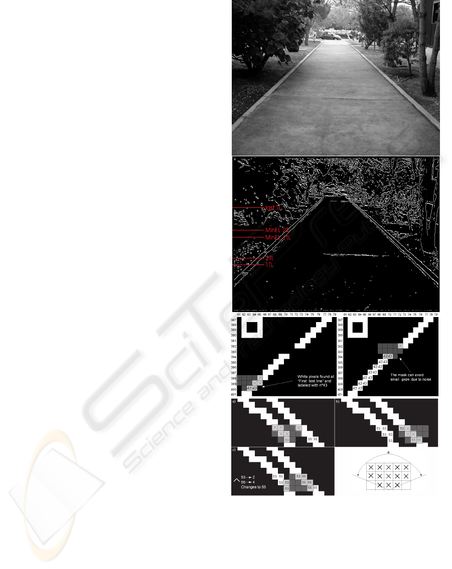
swayed by the user). Figure 1 (top) shows a typical
frame; Fig. 4 shows one of our test sequences.
The system is composed of three processing steps:
(1) Sidewalk border detection and the definition of the
obstacle detection window (ODW). (2) The detection
of obstacles in the ODW using two complementary
processes for tracking irregularities: (i) the number
of local maxima and minima of pixel values, and (ii)
histograms of binary edge information. (3) Tracking
of obstacles in subsequent frames for alerting the user
and obstacle avoidance.
2.1 Sidewalk Border Detection
There are some methods to detect the borders of side-
walks (Kayama et al., 2007). Here we detect them
by using a simple edge detector in combination with
a tracking mask to obtain straight lines, from the bot-
tom of each frame to the top, characterized by slope,
length and proximity to the left and right boundaries
of the frame. The detected borders will define the hor-
izontal position and width of the ODW.
We apply the Canny edge algorithm (Heath et al.,
1997) with three parameters: σ defines the size of the
Gaussian filter, and T
h
and T
l
are the high and low
thresholds for hysteresis edge tracking. We always
use σ = 1.5, T
h
= 0.95 and T
l
= 0.5. Figure 1 (2nd
image from top) shows edges detected in the case of
the frame shown above. Other edge detectors may
perform better, see (Rodrigues and du Buf, 2009), but
most require more CPU time which is critical in this
application.
In order to detect potential sidewalk borders, sev-
eral horizontal test lines are defined in the binary edge
image, I
i
(x,y) with i the frame number. Figure 1 (2nd
image) shows these on the left (in red). On the first
test line “1TL” there are many edge pixels which may
be part of potential border lines. They are starting
points which are labelled differently for the testing
process. A line-tracking mask of size 5x3 (Fig. 1,
bottom-right) is applied to track connected pixels up-
wards, vertically with an opening angle α ≈ 120deg,
from “1TL” to “2TL”, 20 pixels higher, and con-
nected pixels are attributed the same label. Then,
starting at “2TL”, the process is repeated for finding
more potential border lines, complementing the first
search. New labels are generated for pixels on “2TL”
which are not connected to pixels on the first test line.
This second search continues until the last testing line
“last TL”, 200 pixels above “1TL”. Figure 1 (3rd row,
Figure 1: Sidewalk border detection. Top to bottom: an
input frame; edge detection with testing lines indicated (in
red) at the left; start of tracking edge pixels at the first test
line (1 TL) with label 43 (at left) plus the filling of a small
gap (at right); the three steps a, b and c for coping with very
close lines; and the line tracking mask with angle α.
at left) shows the mask tracking edge pixels with label
43 and (at right) tracked edge pixels with a small gap
which will be filled.
Occasionally, there are two or more labeled edge
pixels which are very close. These could correspond
VISAPP 2010 - International Conference on Computer Vision Theory and Applications
236

to a single or to several border lines. In those cases,
when the mask is applied to a new edge pixel, the
already labelled pixels below are checked by using
the vertically mirrored mask. If there are many pixels
with a label not equal to the label of the mask’s central
pixel, the label of the central pixel changes to the one
of the majority of the pixels in the mask. The 4th and
5th rows in Fig. 1 show an example of this process
with steps a, b and c. Final images with connected
and labelled edge pixels are denoted by L
i
(x,y), but
these still contain potential border lines. To be con-
sidered sidewalk borders, detected lines must satisfy
the following three requirements:
(1) Connected edge pixels must have a minimum
length (MinEL) covering at least 80 vertical positions
(MinEL 1TL or MinEL 2TL, depending on the line
starting on 1TL or on 2TL, see Fig. 1, 2nd image from
top). Shorter series are removed.
(2) Connected edge pixels must be almost lin-
ear, i.e., with correlaton r > 0.9, with a slope |b|
between 0.5 and 10. The slope also provides infor-
mation about the sidewalk’s width: the higher the
slope, the narrower the sidewalk. In order to speed
up the correlation/slope process, only eight equidis-
tant points of each potential line are processed. The
correlation r of edge pixels with the same label is
given by r = σ
2
xy
/
q
σ
2
x
· σ
2
y
, where σ
2
xy
is the covari-
ance σ
2
xy
=
∑
xy/n− (
∑
x·
∑
y)/n
2
and σ
2
x
and σ
2
y
are
the variances of x and y
σ
2
x
=
∑
x
2
n
−
∑
x
n
2
;σ
2
y
=
∑
y
2
n
−
∑
y
n
2
. (1)
The regression line is given by L = a+ bx, with
b =
∑
x·
∑
y− n
∑
xy
(
∑
x)
2
− n
∑
x
2
;a =
∑
x·
∑
xy−
∑
y·
∑
x
2
(
∑
x)
2
− n
∑
x
2
. (2)
(3) Occasionally, more than two lines remain as
potential sidewalk borders, or none at all. Depend-
ing on the number of lines n
l
, the following is done:
(i) If no lines are found, n
l
= 0, the last two borders
found in a previous frame will be used. (ii) If a sin-
gle line is found, n
l
= 1, the second line will be au-
tomatically generated, symmetrically with respect to
the vertical line that passes through the intersection
of the line found and the horizontal line through the
vanishing point. The latter is updated dynamically for
each new frame, as explained below. (iii) If two lines
are found, n
l
= 2, they are accepted as sidewalk bor-
ders, but with the following exception: If the signs of
the slopes of the two lines are not different, this means
that we do not have the right lines. The outermost one
is ignored, the innermost one is used, and a new line
is generated as in case n
l
= 1. Here, innermost means
closest to the center of the frame and outermost clos-
est to the left or right frame borders. (iv) In the case
of more lines, n
l
> 2, the most symmetrical and inner
pair of lines is selected.
Above, the vanishing point is used to generate
symmetrical line pairs. At the start of a sequence of
frames, or when no acceptable sidewalk borders can
be detected, the height of the vanishing point will be
initialized at 3/4 of the frame height. Then, when
two correct sidewalk borders are found, the vanish-
ing point is determined by the intersection of the two
borders, and the point is dynamically updated by av-
eraging the points of the previous frame and the new
frame.
After obtaining two valid sidewalk borders, the
obstacle detection window (ODW) is defined for de-
tecting and locating possible obstacles. This window
has predefined upper and a lower limits with a height
of N
v,ODW
= 100 pixels (v is vertical); see Section 2.
The left and right limits are defined by taking 80% of
the distance between the two borders found at the up-
per limit, which gives N
h,ODW
pixels (h is horizontal).
3 OBSTACLE DETECTION AND
AVOIDANCE
For obstacle detection, two different methods are ap-
plied to the ODW. The first one counts variations of
gray values, i.e., local maxima and minima, on each
horizontal line inside the ODW. Then, outliers are re-
duced by averaging counted variations over groups of
lines, and variations over these groups are combined
into a single value which indicates whether the frame
has a possible obstacle or not. Final confirmation is
obtained by combining the results of a few subsequent
frames. The second method is based on irregulari-
ties in vertical and horizontal histograms of the binary
edge image I
i
. An obstacle can lead to two differ-
ent signatures: if the pavement is smooth, an obstacle
may appear as a local excess of edge points, but if
it has a strong texture there will be a huge amount
of edge points and an obstacle may appear as a local
deficiency (lack or gap) of edge points. The second
method is used to confirm the result of the first one,
but it also serves to detect the size and position of an
obstacle in order to guide the user away from it.
3.1 Local Maxima and Minima
(a) A small lowpass filter (averaging block filter of
size 3x3; LP(x, y)) is applied twice to the graylevel
ODW of frame i (F
ODW,i
), so high frequencies are
OBSTACLE DETECTION AND AVOIDANCE ON SIDEWALKS
237

suppressed and a less noisy window can be pro-
cessed. If ∗ denotes convolution, then
˜
F
ODW,i
(x,y) =
F
ODW,i
(x,y) ∗ LP(x,y) ∗ LP(x,y).
(b) Then, the variations of gray values on each hori-
zontal line of the window are computed by applying
the first derivative F
′
ODW,i
(x) = ∂(
˜
F
ODW,i
(x))/∂x.
(c) In order to keep significant variations, a threshold
T
d
= ±2 is applied to the derivative. This suppresses
small transitions and maxima and minima can now
easily be found: where the derivative changes its sign
(zero crossing or ZC), +/− for a maximum and −/+
for a minimum.
(d) The next step consists of counting on each hor-
izontal line y the number of maxima and minima
MM(y) over the ODW window (100 horizontal lines),
MM
i
(y) =
∑
ZC[T
d
[F
′
ODW,i
(x)]].
(e) The result is stabilized by removing outliers.
This is done by taking the average of MM over
triplets of lines, i.e., over three consecutive horizontal
lines, which results in only 33 values for each ODW.
With k = 0, 1,2 and line counting starting at y = 0,
MM
i
(y/3) =
∑
MM
i
(y+ k)/3.
(f) For calculating variations over the ODW’s
lines, the first derivative is applied to MM
i
(y/3),
MM
′
i
(y/3) = ∂(MM
i
(y/3)/∂y.
(g) The last processing step of the ODW of frame i
consists of determining the maximum value (max) of
the absolute value ([·]
+
) of the derivative from step
(f), max
i
= max[MM
′
i
(y/3)]
+
. This value indicates a
possible obstacle in the ODW.
(h) In order to detect and confirm obstacles, a dy-
namic threshold is used to alert the user. The dy-
namic threshold is initialized by computing the av-
erage of max
i
over the first five frames, max =
∑
5
i=1
max
i
/5, and the average of the deviation, i.e.,
the difference between max and each max
i
, dev =
∑
5
i=1
(max
i
− max)/5
+
. The first threshold, T
6
=
max + dev, is going to be tested against max
6
ob-
tained from frame 6, after this frame has been pro-
cessed from step (a) to (g). The same processing is
done with max
i
, dev
i
and T
i
. Two conditions can oc-
cur for i > 5:
(h.1) If max
i
does not exceed threshold T
i
, a new
threshold for the next frame will be calculated by
T
i+1
= 4/5· T
i
+ 1/5 · (max
i
+ dev
i
).
(h.2) Otherwise, a warning-level counter is activated.
If max
i
of the next two frames continue exceeding
the threshold, an obstacle warning will be issued.
The same happens when, after the warning level has
been activated, there is only one frame which does
not exceed the threshold. If more than two consecu-
tive frames do not exceed the threshold, the warning
counter will be reset and the threshold will continue
to be adapted dynamically.
The processing described above detects big vari-
ations of the number of local maxima and minima,
first in the horizontal lines and then over the lines in
the ODW. This allows to detect the appearance and
the disappearance of an obstacle in the window, be-
cause these coincide with the first and last max
i
which
exceed the dynamic threshold. For detecting the po-
sition and size of an obstacle, we apply an analysis of
edge histograms.
3.2 Edge Histograms
This method exploits the already available edge maps
I
i
(x,y), see Section 2.1, but only inside the ODW
I
ODW,i
(x,y). Depending on the smoothness (texture)
of a sidewalk’s pavement, different characteristics are
expected. If r
w
is the fraction of the number of
“white” (edge) pixels N
w,ODW
in I
ODW,i
(x,y), with
N
h,ODW
and N
v,ODW
the window’s dimensions, r
w
=
N
w,ODW
/(N
h,ODW
× N
vODW
).
Extensive tests with real pavements, but without
obstacles, revealed that r
w
> 0.1 indicates rough
surfaces, for example with cobblestones like in
Portuguese-style “calc¸ada,” whereas smaller values
indicate smooth surfaces. In both cases, vertical and
horizontal edge histograms are computed, i.e., for
each line and for each column in the ODW the num-
ber of “white” pixels are summed. Then, the two his-
tograms are smoothed by applying a simple 1D aver-
aging filter.
Two thresholds, T
c
and T
l
, are computed for the
histograms of the lines and columns. For the column
histogram, T
c
is the ratio between the number of white
pixels in the ODW and the number of columns of the
window, T
c
= (N
w,ODW
/N
h,ODW
) × K, and, similarly,
T
l
is the ratio between number of white pixels and the
number of lines, T
l
= (N
w,ODW
/N
v,ODW
) × K, where
K is a normalization factor.
In the case of a smooth pavement (r
w
< 0.1), an
obstacle will appear as an excess of white points, see
Fig. 2, and we apply K = 0.8. An obstacle will be
detected if at least two neighboring values in both the
line and column histograms exceed the thresholds, T
l
and T
c
, respectively.
In the case of a textured pavement (r
w
≥ 0.1), an
obstacle will appear as a lack of white points, see
Fig. 3, and we apply K = 0.4. Now at least two neigh-
boring values in both histograms must be lower than
the corresponding thresholds.
3.3 Obstacle Avoidance
In order to detect an obstacle, both methods described
above must detect something, but in order to save
VISAPP 2010 - International Conference on Computer Vision Theory and Applications
238
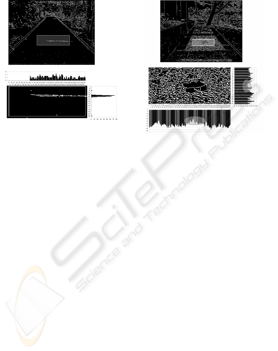
Figure 2: Smooth pavement with a possible obstacle and
corresponding edge histograms.
CPU time the histogram method is only applied to
frames in which the first method has detected some-
thing. Once the histogram method has confirmed the
detection, a sound is generated in order to alert the
user. This sound is modulated such that it indicates
the approximate position and the best way to avoid
the obstacle.
The first method indicates an obstacle somewhere
in the entire ODW. Often, but not always because
it depends on the textures of the pavement and the
object and the latter’s size, the histogram method
can narrow the approximate position to the object’s
bounding box. Blind people prefer to walk near walls
or the fac¸ades of buildings along streets, swaying the
cane in front and keeping contact with the wall or
fac¸ade. Since a wall- and fac¸ade-detection algorithm
has not yet been implemented, we illustrate walking
close to the centerline of paths and sidewalks in this
paper. This scenario is also quite realistic, and avail-
able information about the path’s borders and the van-
ishing point can be used to inform the user about the
centerline. In addition, having the position and di-
mensions (in pixels) of an obstacle’s bounding box,
and the dimensions (in pixels and in meters) of the
ODW, see Section 2, it is easy to convert the bound-
ing box to meters and provide information about the
approximate position and size of the obstacle. If the
obstacle is not centered on the path, the user can be
informed about the left or right side which has the
largest distance between the bounding box and the
path’s left and right borders. In any case, the user
will check the obstacle using the cane.
It should be stressed that the camera is tightly
fixed to the person’s breast such that it points straight
Figure 3: Textured pavement with a possible obstacle and
corresponding edge histograms.
forward, also that the blind have been trained not to
sway much with the body while swaying the cane.
The obstacle-avoidance module requires initial cali-
bration in order to obtain correct distances, for these
depend on each user’s length and posture. In the
future, a disparity module which uses both cameras
of the stereo camera will be integrated. This mod-
ule will complement the obstacle-detection methods
and it will also provide calibrated distance informa-
tion, such that the calibration mentioned above will
no longer be required.
4 CONCLUSIONS AND RESULTS
Various test sequences have been captured on several
paths and sidewalks of Gambelas Campus at the Uni-
versity of the Algarve, with different pavements and
obstacles. Figure 4 shows one sequence with, apart
from the frame number given in the upper-left cor-
ner, the following frame annotation: Type 0 concern
the first 5 initial calibration frames with no obstacles.
Type 1 frames are those in which the variation of max-
ima and minima in the ODW does not exceed the dy-
namic threshold. Type 2 frames do exceed the thresh-
old and the first one activates an alert counter which
counts, from 1 to N, the number of subsequent Type
2 frames. The third alert (N = 3) activates “obstacle
warning” which remains until the first new frame of
Type 1 is encountered.
The first results are very encouraging. The num-
bers of false positives and negatives of the sequences
OBSTACLE DETECTION AND AVOIDANCE ON SIDEWALKS
239

tested were quite small, with more false positives than
false negatives. False positives were mainly caused
by tree leaves and litter, whereas false negatives were
mainly cobblestones pushed up a few centimeters by
tree roots, such that the irregularity of the calc¸ada’s
texture is not detectable.
On a portable computer with an Intel Pentium
clocked at 1.6 GHz, elapsed time to process individ-
ual frames is about 0.5 second. This is already fast
enough for realtime application where the user walks
at normal speed. By using a new portable with a
multi-core processor, more than two frames per sec-
ond can be processed, but the disparity module will
also consume CPU time (although disparity process-
ing might be limited to the ODW), as will other mod-
ules for using GPS in combination with a dedicated
GIS for autonomous navigation.
In general, good results were obtained in the de-
tection of the borders of paths and sidewalks, and
many more paths and sidewalks are now being tested.
Difficulties mainly arise when the color difference or
contrast of a path’s curbs is small, when the curbs
are partly hidden by plants and long grass, or when
a path has no curbs but is delimited by grass or low
shrubs. Similar problems arise in the case of obsta-
cle detection, when the contrast and the texture of an
obstacle and those of the pavement are too similar.
However, most obstacles, including missing cobble-
stones in Portuguese-style “calc¸ada,” the smallest but
most frequent problem, can be detected, but not yet
elevated cobblestones which are being pushed up by
long tree roots. Therefore, detection algorithms must
be improved, even at the cost of more CPU time.
A specific problem is the detection of single and
multiple steps, for which no dedicated algorithm has
been included yet. Occasionally, a wrong obstacle de-
tection window is caused by a wrong detection of the
borders. However, normally this happens in a sin-
gle frame and the problem can be solved by keep-
ing the alert counter counting such that at the next
Type 2 frame an obstacle warning will be issued.
This solution, i.e., tracking information over multiple
frames, can be applied in many more cases. For exam-
ple, positions of borders detected in previous frames
can be extrapolated to new frames in order to narrow
the search area and to confirm the new borders, al-
though sudden and unpredictable movements of the
user cannot be excluded unless they are detected by
big changes of the global optical flow of entire frames.
Such aspects require more research because of the
CPU times which are involved. Also being devel-
oped is a dynamic adaptation of the parameters of the
Canny edge detector as a function of the type of pave-
ment, for resolving finer textures of obstacles like ele-
Figure 4: One test sequence with annotation.
vated cobblestones, but also for the detection of often
minute differences between textures of horizontal and
vertical surfaces of steps when the contrast between
them is too low.
ACKNOWLEDGEMENTS
Portuguese Foundation for Science and Technol-
ogy (FCT) through the pluri-annual funding of
the Inst. for Systems and Robotics (ISR/IST), the
POS Conhecimento Program with FEDER funds, and
FCT project SmartVision (PTDC/EIA/73633/2006).
REFERENCES
Heath, M., Sarkar, S., Sanocki, T., and Bowyer, K. (1997).
A robust visual method for assessing the relative per-
formance of edge-detection algorithms. IEEE Trans.
PAMI, 19(12):1338–1359.
Kayama, K., Yairi, I., and Igi, S. (2007). Detection of
sidewalk border using camera on low-speed buggy.
Proc. IASTED Int. Conf. on Artificial Intelligence
and Applications,13-15 February, Innsbruck, Austria,
pages 262–267.
Kim, L., Park, S., Lee, S., and Ha, S. (2009). An electronic
traveler aid for the blind using multiple range sensors.
IEICE Electronics Express, 11(6):794–799.
Lee, S. and Kang, S. (2008). A walking guidance system
for the visually impaired. Int. J. Pattern Recogn. Artif.
Intell., 22(6):1171 – 1186.
Rodrigues, J. and du Buf, J. (2009). Multi-scale lines and
edges in V1 and beyond: Brightness, object catego-
rization and recognition, and consciousness. BioSys-
tems, 95:206–226.
VISAPP 2010 - International Conference on Computer Vision Theory and Applications
240
