
IMPACT OF A LOSSY IMAGE COMPRESSION ON PARAMETER
ESTIMATION WITH PERIODIC ACTIVE THERMAL IMAGING
Agn
`
es Delahaies
1
, David Rousseau
1
, Laetitia Perez
2
Laurent Autrique
1
and Franc¸ois Chapeau-Blondeau
1
1
Laboratoire d’Ing
´
enierie des Syst
`
emes Automatis
´
es (LISA), Universit
´
e d’Angers
62 avenue Notre Dame du Lac, 49000 Angers, France
2
Laboratoire de Thermocin
´
etique de Nantes, Rue Christian Pauc, 44000 Nantes, France
Keywords:
Image compression, Thermal imaging, Parameter estimation, Material characterization.
Abstract:
Periodic thermal imaging is a method of active thermography based on a periodic thermal stimulation of an
inspected sample material and the analysis of its thermal response when a steady regime is reached. The
original data, a sequence of images sampling the thermal response on a large number of periods, are usually
stored in a raw format. For accurate exploitation of these measurements, the whole sequence of images requires
a significant amount of storage space. In this report, we address the question of the lossy compression of these
sequences of images when they are applied to perform physical parameter estimation. The study investigates
the impact of lossy image compression on the performance of the physical parameter estimation procedure, and
shows the possibility of preserving robust estimation with high compression rate. Perspectives and applications
are then discussed. Performing good enough estimate of physical parameters with compressed images would
permit the use of portable thermal cameras with limited resources in terms of data storage. This would enable
the use of periodic active thermal imaging to perform relatively low cost embedded characterization of thermal
properties of materials.
1 INTRODUCTION
Recent advances (technological improvement, or re-
duction of the production costs) in the domain of pho-
tonic devices, imaging sensors, involving data acqui-
sition, transmission and storage, constitute a stimulat-
ing source of research for information sciences. Re-
cently, there has been the emergence of new types
of nonconventional imaging (polarimetric imaging,
multi-or hyperspectral imaging, ...) which used to be
limited by their capacity of acquisition and storage of
information. Novel domains of application, formerly
restricted by the production costs, have also appeared
for existing imaging systems (MRI or thermal imag-
ing). This context brings forth new configurations and
challenges for the classical signal and image process-
ing operations (detection, estimation, segmentation,
compression, ...).
In this framework, we consider here a task of com-
pression applied to thermal imaging. Introduced in
the 1960’s, thermal imaging uses the Planck law (Lu-
gin, 2008; Breitenstein et al., 2003) which expresses
the luminance of a black body in thermal equilib-
rium at a given wavelength to measure temperatures.
Thermal images poses a practical problem in terms
of compression when long sequences of images are
required. This is specially the case with active ther-
mography methods where the thermal evolution of a
scene is recorded while some external time varying
energy is injected into the scene. There are two main
distinct techniques of active thermal imaging : pulsed
thermal imaging (Lugin, 2008) and periodic thermal
imaging (Breitenstein et al., 2003). The question of
compression has only recently (Lugin, 2008) received
some attention in the domain of active pulsed thermal
imaging. In this report we consider periodic thermal
imaging which, to the best of our knowledge, has not
been yet considered under the scope of compression.
We investigate the impact of a lossy compression on
the performance of a parameter estimation with peri-
odic thermal imaging.
17
Delahaies A., Rousseau D., Perez L., Autrique L. and Chapeau-Blondeau F. (2010).
IMPACT OF A LOSSY IMAGE COMPRESSION ON PARAMETER ESTIMATION WITH PERIODIC ACTIVE THERMAL IMAGING.
In Proceedings of the International Conference on Imaging Theory and Applications and International Conference on Information Visualization Theory
and Applications, pages 17-22
DOI: 10.5220/0002816500170022
Copyright
c
SciTePress
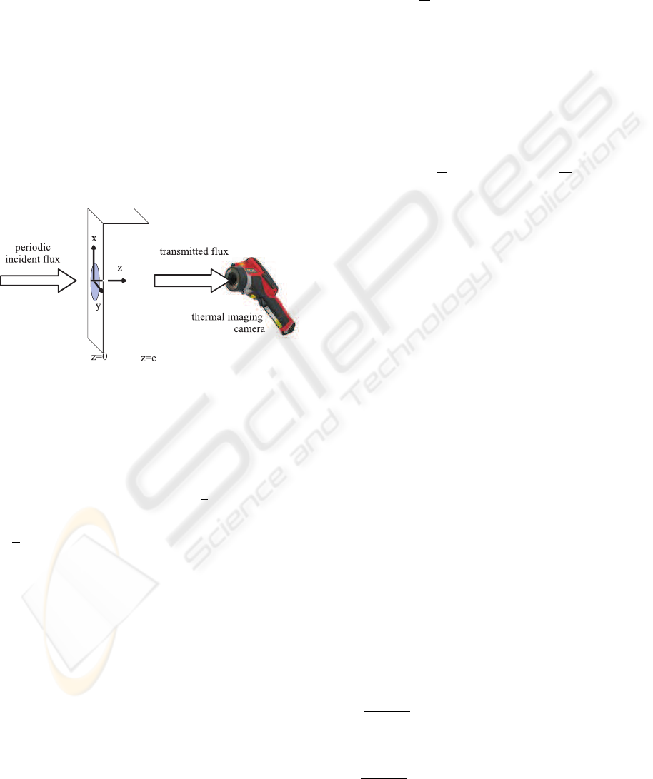
2 PRINCIPLE OF PERIODIC
ACTIVE THERMAL IMAGING
The principe of periodic active thermal imaging is de-
picted in Fig. 1. The setup of Fig. 1 describes the
inspection of a material sample Ω a solid of thick-
ness e. We note X = (x,y, z). The front surface
(Γ
0
: X
0
= (x,y, 0) ∈ Ω) of the sample Ω receives a si-
nusodal radiative flux with angular frequency ω. The
radiative flux Φ : Φ
0
cos(ωt) is spatially centered on
O = (0, 0, 0) and is uniform over a disk of radius R and
zero outside this disk. If the radiative flux is absorbed
by the material, the resulting heat diffuses inside the
material. When the diffused heat arrives on the op-
posite side (Γ
e
: X
e
= (x,y, e) ∈ Ω) a flux is radiated.
A thermal imaging camera is placed on the opposite
side to the incident radiative flux source and receives
a transmitted radiative flux.
Figure 1: Principe of periodic active thermal imaging for
the inspection of a material sample Ω of thickness e.
The camera then uses the Planck law to calculate
the surface temperature on Γ
e
from this transmitted
radiative flux. When the steady periodic regime is
reached, the temperature in the sample Ω and on the
opposite side Γ
e
is θ(X,t) = R e{θ(X,t)} (Breiten-
stein et al., 2003) with
θ(X,t) = θ
DC
(X)+ M(X)exp( jωt)exp( jϕ(X)) ,
(1)
where θ
DC
(X) is the average temperature at X, M(X)
is the modulus image of the thermal oscillations
which depicts the spatial attenuation of the incident
heat flux in the material sample, and ϕ(X) the phase
image which represents the delay between the inci-
dent and the transmitted heat flux due to the material
sample. Both images M(X) and ϕ(X ) thus carry in-
formation on the thermal properties of the material.
A specific interest of the phase ϕ(X) is that it does
not depend on the knowledge of the sample emissiv-
ity (Breitenstein et al., 2003). In the following we will
thus only use the phase ϕ(X) to analyze the thermal
behavior of the sample.
There are various experimental sources of noise
in the phase image ϕ(X) including spurious high fre-
quency components in the excitation and electronic
noise on the thermal cameras. Therefore, high ac-
curacy measurement of ϕ(X) requires heavy statis-
tics. A sequence of N thermal images θ(X ,n) with
n ∈ [0, N −1] is usually acquired to cover a large num-
ber of periods
2π
ω
with a high frequency rate (typically
of some 50 images per period). If we assume the noise
in θ(X,n) to be Gaussian, the maximum likelihood
estimator
ˆ
ϕ(X) of image ϕ(X) can be shown to be ap-
proximately for large N (Kay, 1993)
ˆ
ϕ(X) = arctan
µ
−
β
2
(X)
β
1
(X)
, (2)
with
β
1
(X) =
2
N
N−1
∑
n=0
θ(X,n)cos
µ
ω
n
F
e
, (3)
and
β
2
(X) =
2
N
N−1
∑
n=0
θ(X,n)sin
µ
ω
n
F
e
. (4)
An example of phase
ˆ
ϕ(X) evaluated from the exper-
imental setup of Fig. 2 is visible in Fig. 3. As ex-
plained in Fig. 2, the amount of memory required to
produce Fig. 3 with a good accuracy is huge.
In the following, we are going to show how it is
possible to use the phase images ϕ(X ) of Fig. 3 to
perform estimation of a physical parameter in a ma-
terial. We will then compare the performance of this
estimate with a periodic active thermal imaging se-
quence applied on raw thermal images θ(X, n) and on
the same sequence after a lossy compression.
3 APPLICATION TO
PARAMETER ESTIMATION
Periodic active thermal imaging as described in sec-
tion 2 can be applied to perform physical parameter
estimation of a material. This requires the modeling
of the sample response of Fig. 2 which can be done in
the following way (Perez and Autrique, 2009). Tem-
perature θ(X ,t) in the material sample Ω, assumed
here homogeneous and isotropic, follows from heat
diffusion equation
α
∂θ(X,t)
∂t
− ∆θ(X,t) = 0 ,∀(X,t) ∈ Ω × T , (5)
and boundary conditions on Γ
0
λ
∂θ(X,t)
∂z
= hθ(X ,t) − Φ ,∀(X,t) ∈ Γ
0
× T , (6)
IMAGAPP 2010 - International Conference on Imaging Theory and Applications
18
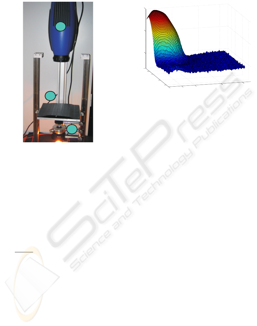
3
2
1
Figure 2: Experimental setup of periodic active thermal
imaging used to perform the analysis. The material sam-
ple (sticker 2) taken as reference is a plate of titanium of
thichness e = 1 mm. This sample is placed in the focal
plane of a K
¨
ohler lightning device (sticker 1) which pro-
duces a uniform flux on a circular disk of radius R = 2.5
mm. The incident radiative flux is produced by an halo-
gen lamp (36V-400W) placed under the sample and con-
trolled by a on/off switch of angular frequency ω = 5.66
rad.s
−1
. Thermal images θ(X,n) are acquired by a SC5000
FLIR thermal camera (sticker 3) at the sampling frequency
F
e
= 50 Hz with format 320 × 256 coded on 14 bits. The
phenomenon is recorded on 18 periods. This produce a file
of 999 images representing 1.67 Go to be stored.
on Γ
e
λ
∂θ(X,t)
∂z
= hθ(X ,t) , ∀(X ,t) ∈ Γ
e
× T , (7)
and initial temporal condition θ(X ,0) = 0 ∀(X) ∈ Ω.
Physical parameters of the modeling of Eqs. (5)-(7)
are the diffusivity α in [m
2
.s
−1
], the convective coeffi-
cient h in [W.m
−2
.K
−1
] and the conductivity λ = αρc
in [W.m
−1
.K
−1
] where ρ is the density in [kg.m
−3
]
and c the specific heat in [J.kg
−1
.K
−1
]. Resolution
of Eqs. (5)-(7) provides the temperature θ(X,t) in
the whole material Ω. It is then possible to confront
the temperature θ(X,t) on the surface of the side Γ
e
measured by the thermal imaging and deduced by the
model of Eqs. (5)-(7). One can use this experiment-
model confrontation to estimate the value of an un-
known parameter. In the general case, there exists no
exact analytical explicit expressions for ϕ(X). The
solution of Eqs. (5)-(7) can be numerically performed
0
5
10
20
30
0
5
10
20
30
−600
−300
0
phase in °
Figure 3: Phase ϕ(X ) evaluated with Eqs. (2)-(4) from raw
images acquired with experimental setup and material sam-
ple described in Fig. 2. The phase plotted as a function of
position (x,y) in mm has been unwrapped with the standard
Itoh’s algorithm (Ghiglia and Pritt, 1998).
by the method of (Perez and Autrique, 2009). We
show in Fig. 4 an example of confrontation of an
experimental phase ϕ(X) obtained with the setup of
Fig. 1 and the algorithm of Eqs. (2)-(4) with the nu-
merical resolution of Eqs. (5)-(7). In Fig. 4, the un-
known parameter is the conductivity λ. The estimated
value (given in Table 1 for the material of Fig. 2)
is chosen as the one which minimizes the average
quadratic error between the phase ϕ(X) in experi-
ments and in the numerical solution of Eqs. (5)-(7).
In Fig. 4, the parameter estimation has been per-
formed on raw data. We will now compare with the
estimation when the algorithm of Eqs. (2)-(4) is per-
formed on compressed images.
4 INFLUENCE OF A LOSSY
COMPRESSION
To illustrate our methodology in assessing the impact
of a lossy compression of images on physical param-
eters estimation, we choose one lossy compression
technique usually implemented by default in ther-
mal cameras. A reasonable choice (Bovik, 2000) is
the standard JPEG compression. Temperature images
θ(X,n) are coded on 14 bits with the camera pre-
sented in Fig. 2. The standard JPEG compression
codes images on 8 bits. Therefore, requantization (al-
ready bringing a 2
14
/2
8
compression factor) and nor-
malization are necessary before the JPEG compres-
sion step is applied. For each image θ(X,n) of the
acquired sequence, the maximum θ
max
and minimum
θ
min
temperature over the whole sequence are stored
separately and an intermediate 8-bit gray level image
IMPACT OF A LOSSY IMAGE COMPRESSION ON PARAMETER ESTIMATION WITH PERIODIC ACTIVE
THERMAL IMAGING
19
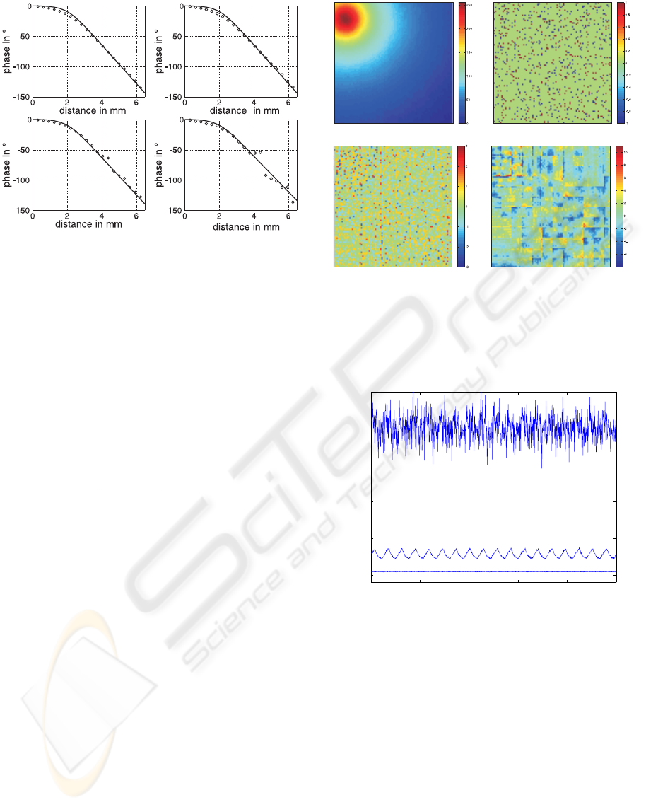
C D
A B
Figure 4: Phase as a function of distance. Solid line
is the numerical solution of Eqs. (5)-(7) with α = 9.3 ×
10
−6
m
2
.s
−1
, h = 20 W.m
−2
.K
−1
, ρ = 4507 kg.m
−3
, c =
520 J.kg
−1
.K
−1
. Circles stand for the experimental points
obtained from the setup of Fig. 2. By comparison with
Fig. 3, the analysis is performed on a line starting at the
maximum heating point in the modulus image M(X,t) taken
as phase reference. (A) is for a phase calculated with raw
images directly acquired by the thermal camera. (B)(C)(D)
is for a phase calculated with images after a JPEG compres-
sion with compression parameter CMP of section 4 respec-
tively equal to 100, 90 and 25. The conductivity estimated
from each panel (A)-(D) are visible in Table 1.
I(X ,n) is created with
I(X ,n) =
255
θ
max
− θ
min
(θ(X,n)− θ
min
) . (8)
A standard JPEG compression is then applied to
I(X ,n) to create the compressed sequence of images
I
CMP
(X,n). We used the JPEG compression available
in the programming language Matlab (version 7) with
a compression parameter CMP in the range [1-100]
for varying the quality/size ratio. The value 100 for
CMP corresponds to high quality at low compression
and 1 to low quality at high compression. A visual ap-
preciation of the typical impact of the distorsion due
to this JPEG compression is visible in Fig. 5. For an
uncompressed raw image I(X,n) in Fig. 5A consid-
ered at a given instant n, Fig. 5 displays, for various
values of the compression parameter CMP, the error
image ε(X,n) defined as
ε(X,n) = I(X,n)− I
CMP
(X,n) . (9)
A possible way to quantify the distorsion due to
the lossy compression is to calculate a spatial mean
square error for each sample n
MSE(n) = hε(X,n)i
X
. (10)
Temporal evolutions of MSE of Eq. (10) are given in
Fig. 6.
A
C
D
C
B
Figure 5: Panel A : uncompressed raw image I(X,n) of tem-
perature coded on 256 digital levels according to Eq. (8).
Panels (B,C,D) : error images ε(X, n) of Eq. 9 for decreas-
ing compression parameter CMP respectively equal to 100,
90, 25 and corresponding compression rates indicated in Ta-
ble 1.
0 200 400 600 800 1000
0
0.5
1
1.5
2
2.5
sample n
mean square error MSE
Figure 6: Mean square error MSE of Eq. (10) temporal
evolutions along the 999 images acquired with the setup of
Fig. 2 after JPEG compression. From bottom to up the com-
pression parameter CMP is respectively equal to 100, 90,
25.
It is possible from Fig. 5 and Fig. 6 to figurate how
both spatial and temporal noise will disturb the im-
age sequence. However, distorsion measured by the
mean square error does not assess the impact of the
compression on the useful information carried by the
sequence concerning the parameter to be estimated.
This type of questioning also arises when the per-
ceived distorsion due to a lossy compression is ap-
preciated by the human vision. Psychovisual experi-
ments are requested in this case. Here, since we are
in a measurement context, we can objectively address
IMAGAPP 2010 - International Conference on Imaging Theory and Applications
20

the quantitative impact of the distorsion on the qual-
ity of the measure. To this end, we now perform the
parameter estimation procedure of section 3 on the
sequence of images I
CMP
(X,n) for several values of
the compression rate controlled by the compression
parameter CMP. The results, visible in Table 1, show
how the quality of the estimate is affected by the lossy
compression. The CMP coefficient acts on the size of
the imagette used to perform the JPG compression.
For low values of parameter CMP (in Fig. 4D) some
discontinuities due to these imagette are clearly vis-
ible. Nevertheless, thermal images θ(X,n) are vary-
ing very smoothly in the spatial domain. JPEG al-
gorithm acts like a low-pass filter for spatial frequen-
cies which tends to preserve the low frequencies of
θ(X,n). Therefore, it appears that for sufficiently low
(up to 66%) compression rate the compression distor-
tion on each individual image barely has no effect on
the useful information carried by the whole sequence.
As demonstrated in Table 1, the estimation error by
comparison with raw datas increases slower than the
compression rate decreases. The measurement allows
to perform identification of the class of material in
terms of thermal properties even at very high com-
pression rate.
Table 1: Estimate of the conductivity λ of the ma-
terial sample of Fig. 2 in [W.m
−1
.K
−1
] performed af-
ter lossy JPEG compression at various rate (CR =
size(I
CMP
(X, n))/size(θ(X,n)). As a comparison, the typ-
ical λ for titanium is expected in the range 5 to 25
W.m
−1
.K
−1
depending on the purity of the material. As
an order of magnitude thermal conductivity of pure copper
is 401 W.m
−1
.K
−1
and pure aluminium is 237 W.m
−1
.K
−1
CR CMP estimate relative error
raw 21.42 0 %
66% 100 21.41 0.04%
88% 90 23.24 8.54%
94% 25 25.88 20.8%
5 CONCLUSIONS
In this report we have shown and analyzed quanti-
tatively the robustness of parameter estimation with
periodic active thermal imaging toward lossy JPEG
compression. An originality in our approach by com-
parison with the recent work of (Lugin, 2008) is that
we have not considered the distortion due to lossy im-
age compression on the thermal images but directly
on the quantitative information they carry. This ap-
proach is interesting in general for quantitative phys-
ical imaging since it shows the possibility of condi-
tions where lossy image compression can entail al-
most no loss in the information extracted form the im-
age.
Further development of this work is to consider
video-compression algorithms (Shi and Sun, 2000)
to compress the whole sequence of images. In-
stead of compressing each image separately, video-
compression treats groups of successive pictures.
This video compression would enable higher com-
pression rates and bring additional distortion on the
information carried on each pixel with time. Other
ways to reduce the amount of data required by peri-
odic active thermal imaging are also to decrease the
sampling frequency, the imaging sensor dynamic and
the number of pixels. It would then be interesting
to see how these configurations together with video
lossy compression degrade the quality of the estimate
of physical parameters. For illustration in this re-
port, the unknown parameter to be estimated was the
conductivity. The sensitivity to compression distor-
sion could also depend on the parameter to be esti-
mated and it would also be important to explore this
systematically while investigating other compression
schemes.
Typical limit to look for in terms of compression
would be in the direction of the technical character-
istics of the new portable thermal cameras which are
now available at relative low cost. An MPEG video
flux is usually available as an output of these cam-
eras. This facility is initially thought as a qualitative
tool enabling the display of thermal images on screens
larger than the screen of the camera itself. Yet, as il-
lustrated in this report, periodic active thermal imag-
ing only requires the relative spatial and temporal
variations of the gray levels to perform quantitative
measurement. An application of our results would
therefore be to evaluate the possible usefulness of
these portable thermal cameras for quantitative peri-
odic active thermal imaging.
ACKNOWLEDGEMENTS
Authors would like to thank Patrice BALCON and
Franck CARETTE from FLIR Systems for useful dis-
cussions.
REFERENCES
Bovik, A. C. (2000). Handbook of Image and Video Pro-
cessing. Academic Press, New York.
Breitenstein, O., Warta, W., and Langenkamp, M. (2003).
Lock-in Thermography. Springer, New York.
IMPACT OF A LOSSY IMAGE COMPRESSION ON PARAMETER ESTIMATION WITH PERIODIC ACTIVE
THERMAL IMAGING
21

Ghiglia, D. C. and Pritt, M. D. (1998). Two Dimensional
Phase Unwrapping : Theory, Algorithm and Software.
Wiley, New York.
Kay, S. M. (1993). Fundamentals of Statistical Signal Pro-
cessing: Estimation Theory. Prentice Hall, Engle-
wood Cliffs.
Lugin, S. (2008). Pulsed Thermography. VDM Verlag,
New York.
Perez, L. and Autrique, L. (2009). Robust determination of
thermal diffusivity values from periodic heating data.
Inverse problems, 25:2310–2313.
Shi, Y. Q. and Sun, H. (2000). Image and Video Compres-
sion for Multimedia Engineering. CRC Press, New
York.
IMAGAPP 2010 - International Conference on Imaging Theory and Applications
22
