
REAL-TIME MOVING OBJECT DETECTION IN VIDEO
SEQUENCES USING SPATIO-TEMPORAL ADAPTIVE GAUSSIAN
MIXTURE MODELS
Katharina Quast, Matthias Obermann and Andr´e Kaup
Multimedia Communications and Signal Processing, University of Erlangen-Nuremberg
Cauerstr. 7, 91058 Erlangen, Germany
Keywords:
Object detection, Background modeling.
Abstract:
In this paper we present a background subtraction method for moving object detection based on Gaussian
mixture models which performs in real-time. Our method improves the traditional Gaussian mixture model
(GMM) technique in several ways. It takes into account spatial and temporal dependencies, as well as a
limitation of the standard deviation leading to a faster update of the model and a smoother object mask. A
shadow detection method which is able to remove the umbra as well as the penumbra in one single processing
step is further used to get a mask that fits the object outline even better. Using the computational power of
parallel computing we further speed up the object detection process.
1 INTRODUCTION
The detection of moving objects in video sequences is
an important and challenging task in multimedia tech-
nologies. Most detection methods follow the princi-
ple of background subtraction. To segment moving
foreground objects from the background a pure back-
ground image has to be estimated. This reference
background image is then subtracted from each frame
and binary masks with the moving foreground objects
are obtained by thresholding the resulting difference
images.
In (Stauffer and Grimson, 1999; Power and
Schoonees, 2002) the values of a particular pixel over
time are modeled as a mixture of Gaussian distri-
butions. Thus, the background can be modeled by
a Gaussian mixture model (GMM). Once the pixel-
wise GMM likelihood is obtained, the final binary
mask is either generated by thresholding (Stauffer and
Grimson, 1999; Power and Schoonees, 2002; Kaew-
TraKulPong and Bowden, 2001) or according to more
sophisticated decision rules (Carminati and Benois-
Pineau, 2005; Li et al., 2004; Yang and Hsu, 2006).
Although the Gaussian mixture model technique is
quite successful the obtained binary masks are often
noisy and irregular. A main reason for this is that spa-
tial and temporal dependencies are neglected in most
approaches. In (Li et al., 2004) a Bayesian frame-
work for object detection is proposed that incorpo-
rates spectral, spatial, and temporal features. But the
spatial dependency is only deployed during post pro-
cessing mainly by applying morphological operations
which leads to poor object contours.
We improvethe standard GMM method by regard-
ing spatial and temporal dependencies and integrating
a limitation of the standard deviation into the tradi-
tional method. Combining this improved method with
our fast shadow removal technique, which is inspired
by the technique of (Porikli and Tuzel, 2003), leads to
good binary masks without adding any complex and
computational expensive extensions to the method.
Thus, better masks are obtained while the computa-
tional speed of the standard GMM method is kept and
further post processing can be omitted. Through par-
allelization of the algorithm we even achieve an enor-
mous performance speedup.
In the follwing, an overview of the GMM method
is given in Section 2. In Section 3 the proposed
method is first described explaining the use of spatial
and temporal dependencies, the limitation of the stan-
dard deviation, and the shadow removal technique.
Experimental results and implementation issues are
discussed in Section 4. Finally conclusions are drawn
in Section 5.
413
Quast K., Obermann M. and Kaup A. (2010).
REAL-TIME MOVING OBJECT DETECTION IN VIDEO SEQUENCES USING SPATIO-TEMPORAL ADAPTIVE GAUSSIAN MIXTURE MODELS.
In Proceedings of the International Conference on Computer Vision Theory and Applications, pages 413-418
DOI: 10.5220/0002816904130418
Copyright
c
SciTePress

2 GMM OVERVIEW
As proposed in (Stauffer and Grimson, 1999) each
pixel in a scene can be modelled by a mixture of K
Gaussians. The modelling is based on the estimation
of the probability density of the color value for each
pixel. It is assumed that the color value of a given
pixel is determined by the surface of an object which
is in the view of the concerned pixel. In non-static
scenes up to K different objects k = 1...K might come
into the view of a pixel. Therefore, in a monochro-
matic video sequence the probability density of the
color value c of a pixel x caused by an object k can be
expressed as a Gaussian function with mean µ
k
and
standard deviation σ
k
η(c,µ
k
,σ
k
) =
1
√
2πσ
k
e
−
1
2
(
c−µ
k
σ
k
)
2
(1)
In case of more than one color channel the probability
density of the color value of a pixel is
η(c,µ
µ
µ
k
,Σ
k
) =
1
(2π)
n
2
|Σ
k
|
1
2
e
−
1
2
(c−µ
µ
µ
k
)
T
Σ
−1
k
(c−µ
µ
µ
k
)
(2)
where c is the color vector and Σ is a n-by-n covari-
ance matrix of the form Σ
k
= σ
2
k
I, because it is as-
sumed that the RGB color channels have the same
standard deviation and are independent from each
other. While the latter is certainly not the case, by this
assumption a costly matrix inversion can be avoided
at the expense of some accuracy.
The probability of a certain pixel x in frame t hav-
ing the color value c is the weighted mixture of the
probability densities of the k = 1...K objects
P(c
t
) =
K
∑
k=1
ω
k,t
·η(c
t
,µ
µ
µ
k,t
,Σ
k,t
) (3)
with ω
k
as the weight for the respective Gaussian dis-
tribution. For practical reasons K is limited to a small
number from 3 to 5. For each new frame of the video
sequence the existing model has to be updated. Af-
ter that a background image is estimated based on
the model and the image can be segmented into fore-
ground and background. To update the model it is
checked if the new pixel color matches one of the ex-
isting K Gaussian distributions. A pixel x with color
c matches a Gaussian k if
|c−µ
µ
µ
k
| < d ·σ
k
(4)
where d is a user defined parameter. If c matches a
distribution the model parameters are adjusted as fol-
lows:
ω
k,t
= (1−α)ω
k,t−1
+ α (5)
µ
µ
µ
k,t
= (1−ρ
k,t
)µ
µ
µ
k,t−1
+ ρ
k,t
c
t
(6)
σ
k,t
=
q
(1−ρ
k,t
)σ
2
k,t−1
+ ρ
k,t
(kc
t
−µ
µ
µ
k,t
k)
2
(7)
where ρ
k,t
= α/ω
k,t
according to (Power and
Schoonees, 2002). For unmatched distributionsonly a
new ω
k,t
has to be computed following equation (17).
ω
k,t
= (1−α)ω
k,t−1
(8)
The other parameters remain the same. The Gaussians
are now ordered by the value of the reliability measure
ω
k,t
/σ
k,t
in such a way that with increasing subscript
k the reliability decreases. If a pixel matches more
than one Gaussian distribution the one with the most
reliability is choosen. If the constraint in equation (4)
is not complied and a color value can not be assigned
to any of the K distributions, the least probable dis-
tribution is replaced by a distribution with the current
value as its mean value, a low prior weight and an
initally high standard deviation and ω
k,t
is rescaled.
A color value is regarded to be background with
higher probability (lower k) if it occurs frequently
(high ω
k
) and does not vary much (low σ
k
). To de-
termine the B background distributions a user defined
prior probability T is used
B = argmin
b
b
∑
k=1
w
k
> T
. (9)
The rest K −B distributions are foreground.
3 PROPOSED METHOD
3.1 Temporal Dependency
The traditional method takes into account only the
mean temporal frequency of the color values of the
sequence. The more often a pixel has a certain color
value, the greater is the probability of occurrence of
the corresponding Gaussian distribution. But the di-
rect temporal dependency is not taken into account.
To detect the static background regions and to en-
hance adaption of the model to these regions a param-
eter u is introduced to measure the number of cases
where the color of a certain pixel was matched to the
same distribution in subsequent frames
u
t
=
(
u
t−1
+ 1, if k
t
= k
t−1
0 else
(10)
where k
t−1
is the distribution which matched the pixel
color in the previous frame and k
t
is the current Gaus-
sian distribution. If u exceeds a threshold u
min
the
factor α is multiplied by a constant s > 1
α
t
=
(
α
0
·s, if u
t
> u
min
α
0
else
(11)
VISAPP 2010 - International Conference on Computer Vision Theory and Applications
414
(a) (b)
(c)
(d)
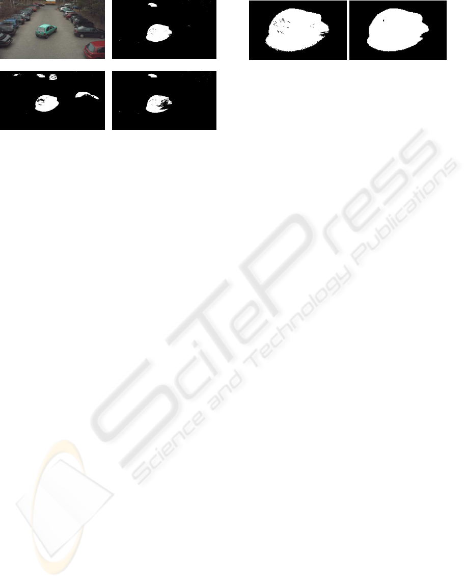
Figure 1: A frame of sequence Parking and the correspond-
ing detection results of the proposed method compared to
the traditional method. First row: original frame (a) and
background estimated by the proposed method with tempo-
ral dependency (α
0
= 0.001, s = 10, u
min
= 15) (b). Bottom
row: standard method with α = 0.001 (c) and α = 0.01 (d).
The factor α
t
is now temporal dependent and α
0
is
the initial user defined α. In regions with static im-
age content the model is now faster updated as back-
ground. Since the method doesn’t depend on the pa-
rameters σ and ω, the detection is also ensured in un-
covered regions. In the top row of Figure 1 the orig-
inal frame of sequence Parking and the correspond-
ing background estimated using GMMs combined
with the proposed temporal dependency approach is
shown. The detection results of the standard GMM
method with different values of α are shown in the
bottom row of Figure 1. While the standard method
either detects a lot of false positives or false negatives,
the method considering temporal dependency obtains
quite a good mask.
3.2 Spatial Dependency
In the standard GMM method each pixel is treated
separately and spatial dependency between adjacent
pixels is not considered. Therefore, false positives
caused by noise based exceedance of d ·σ
k
in equa-
tion (4) or slight lighting changes are obtained. Since
the false positives of the first type are small and iso-
lated image regions the ones of the second type cover
larger adjacent regions as they mostly appear at the
border of shadows, the so called penumbra. Through
spatial dependency both kinds of false positives can
be eliminated.
Since in the case of false positives the color value
c of x is very close to the mean of one of the B dis-
tributions, at least for one distribution k ∈ [1...B] a
small value is obtained for |c −µ
µ
µ
k
|. In general this
is not the case for true foreground pixels. Instead of
generating a binary mask we create a mask M with
weighted foreground pixels. For each pixel x = (x, y)
Figure 2: Detection result of the proposed method with tem-
poral dependency (left) compared to the proposed method
with temporal and spatial dependencies (right) for sequence
Parking.
its weighted mask value is estimated according to the
following equation
M(x) =
0, if k(x) ∈ [1...B]
min
k=[1...B]
(|c−µ
µ
µ
k
|) else
(12)
The background pixels are still weighted with zero,
while the foreground pixels are weighted according
to the minimum distance between the pixel and the
mean of the background distributions. Thus, fore-
ground pixels with a larger distance to the background
distributions get a higher weight. To use the spatial
dependency as in (Aach and Kaup, 1995), where the
neighborhood of each pixel is considered, the sum of
the weights in a square window W is computed. By
using a threshold M
min
the number of false positives
is reduced and a binary mask BM is estimated from
the weighted mask M according to
BM(x) =
(
1, if
∑
W
M(x) > M
min
0 else
(13)
In Figure 2 (right) part of a binary mask for se-
quence Parking obtained by GMM method consider-
ing temporal as well as spatial dependency is shown.
3.3 Avoiding Typical Detection
Artefacts
If a pixel in a new frame is not described very well by
the current model, the standard deviation of a Gaus-
sian distribution modelling the foreground might in-
crease enourmously. This happens most notably when
the pixel’s color value deviates tremendouslyfrom the
mean of the distribution and large values of c−µ
µ
µ
k
are
obtained during the model update. The larger σ
k
gets
the more color values can be matched to the Gaussian
distribution. Again this increases the probability of
large values of c−µ
µ
µ
k
.
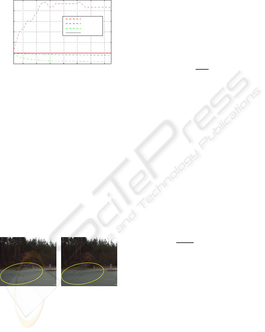
Figure 3 illustrates the changes of the standard de-
viation over time for the first 150 frames of sequence
Street modeled by 3 Gaussians. The minimum, mean
and maximum standard deviationsof all Gaussian dis-
tributions for all pixels are shown (dashed lines). The
REAL-TIME MOVING OBJECT DETECTION IN VIDEO SEQUENCES USING SPATIO-TEMPORAL ADAPTIVE
GAUSSIAN MIXTURE MODELS
415
frame no.
standard deviation σ
σ
max
σ
mean
σ
min
σ
0
20 40 60 80 100 120 140
0.4
0
10
20
30
40
50
60
Figure 3: Maximum, mean and minimum standard devia-
tion of all Gaussian distribution of all pixels for the first
150 frames of sequence Street.
maximum standard deviation increases over time and
reaches high values. Hence, all pixels which are not
assigned to one of the other two distributions will be
matched to the distribution with the large σ value.
The probability of occurrence increases and the dis-
tribution k will be concidered as a background distri-
bution. Therefore, even foreground colors are easily
but falsely identified as background colors. Thus, we
suggest to limit the standard deviation to the initial
standard deviation value σ
0
as demonstrated in Fig-
ure 3 by the continuous red line. In Figure 4 the tra-
ditional method (left background) is compared to the
one where the standard deviation is restricted to the
initial value σ
0
(right background). By examining the
two backgrounds it is clearly visible that the limita-
tion of the standard deviation improves the quality of
the background model, as the dark dots and regions
in the left background are not contained in the right
background.
Figure 4: Background estimated for frame 97 of sequence
Street without (left) and with limited standard deviation
(right). Ellipse marks region, where detection artefacts are
very likely to occur.
3.4 Single Step Shadow Removal
Even though the consideration of spatial dependency
can avert the detection of most penumbra pixels, the
pixels of the deepest shadow, the so called umbra,
might still be detected as foreground objects. Thus,
we combined our detection method with a fast shadow
removal scheme inspired by the method of (Porikli
and Tuzel, 2003).
Since a shadow has no affect on the hue, but
changes the saturation and decreases the luminance,
possible shadow pixels can be determined as follows.
To find the true shadow pixels, the luminance change
is computed in the RGB space by projecting the color
vector c onto the background color value b
h =
hc,bi
|b|
(14)
A luminance ratio is defined as r = |b|/h to measure
the luminance difference between b and c while the
angle φ = arccos(h/c) between the color vector c and
the background color value b measures the saturation
difference. Each foreground pixel is classified as a
shadow pixel if the following two terms are both stat-
isfied
r
1
< r < r
2
, φ < φ
1
(15)
where r
1
is the maximum allowed darkness, r
2
is the
maximum allowed brightness and φ
1
is the maximum
allowed angle separation. Since umbra pixels are
considerably darker than penumbra pixels the condi-
tions for penumbra and umbra suppression can not be
satisfied simultaneously. Thus, the shadow removal
scheme described in (Porikli and Tuzel, 2003) has to
be run twice with different values for r
1
, r
2
and φ
1
to
remove either penumbra or umbra.
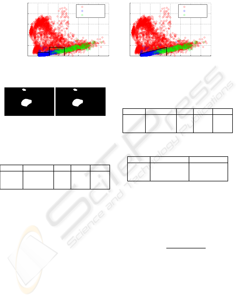
In the φ-r-plane the area were shadow is removed
is represented by two rectangles as shown in the left
graph of Figure 5. To reduce the processing time we
introduce a second angle φ
2
and the angle constraint
of equation (15) is replaced by
φ <
φ
2
−φ
1
r
2
−r
1
·(r−r
1
) + φ
1
. (16)
a new shadow detection area is defined in the φ-r-
plane as can be seen in the right graph of Figure 5.
Thus, umbra and penumbra can be removed reason-
ably well in one single step instead of two separated
ones. To clearly show the performance, both shadow
removal approaches were applied on the results of
Subsection 3.2. The obtained masks are shown in Fig-
ure 6.
4 IMPLEMENTATION AND
EXPERIMENTAL RESULTS
The proposed algorithm has been tested on several
video sequences. After parameter testing we obtained
good detection results for the sequences applying the
VISAPP 2010 - International Conference on Computer Vision Theory and Applications
416
r
φ in degree
object
penumbra
umbra
0.5 1 1.5
2
2.5 3 3.5 4 4.5
0
5
10
15
20
25
r
φ in degree
object
penumbra
umbra
0.5 1 1.5
2
2.5 3 3.5 4 4.5
0
5
10
15
20
25
Figure 5: Detection areas (black rectangles) for umbra and penumbra removal in φ-r-plane using the two-step method (left)
and detection area (black triangle) for shadow removal (umbra and penumbra) in φ-r-plane using the one-step method (right).
Figure 6: The proposed one-step shadow removal tech-
nique achieves the same result(left) as the two-step method
(right), while it needs only half the processing time.
Table 1: Average detection rate R
D
, average false positives
rate R
FP
and average false negatives rate R
FN
using the tra-
ditional GMM method.
sequence no. of frames R
D
(%) R
FP
(%) R
FN
(%)
Parking 20 98.72 1.11 0.17
Shopping 20 95.65 3.40 0.95
Airport 20 95.35 2.56 2.09
GMM method with K = 3, T = 0.7, α
0
= 0.002,
d = 2.5 and σ
0
= 10, while setting the parameters for
temporal dependency u
min
= 15 and s = 10 and the
parameters for spatial dependency to M
min
= 180 and
W = 3 ×3. One-step shadow removal was run with
r
1
= 1, r
2
= 1.7, φ
1
= 4 and φ
2
= 6. For sequences
Shopping and Airport the binary masks of the pro-
posed method are compared with the results of the tra-
ditional GMM method (Stauffer and Grimson, 1999)
and the statistical background modeling method of
(Li et al., 2004) in Figure 7. The visual study of the
masks shows that the proposed method generates rea-
sonably good detection results which can even outper-
form methods with more complicated detection rou-
tines. To further evaluate the detection performance a
detection rate R
D
and a false alarm rate for the false
positives R
FP
and the false negatives R
FN
were cal-
culated for each frame and then averaged over the
whole sequence. For computing R
D
, R
FP
and R
FN
the
mask is compared with a ground truth. False positives
are defined as the number of background pixels that
are misdetected as foreground while false negatives
Table 2: Average detection rate R
D
, average false positives
rate R
FP
and average false negatives rate R
FN
using the pro-
posed method.
sequence no. of frames R
D
(%) R
FP
(%) R
FN
(%)
Parking 20 99.29 0.50 0.21
Shopping 20 97.56 1.43 1.01
Airport 20 95.88 2.07 2.06
Table 3: F
1
scores of the traditional GMM method and the
proposed method.
sequence traditional GMM proposed method
Parking 0.76 0.85
Shopping 0.70 0.81
Airport 0.65 0.68
are the number of missing foreground pixels. For se-
quences Shopping and Airport the ground truths from
(Li et al., 2004) were used while the ground truths for
sequence Parking were manually labeled.
By comparing the detection rates it is obvious that
the proposed method (Table 2) outperforms the tradi-
tional method (Table 1). We further calculated the F
1
measure (Table 3) for sequence Airport:
F
1
= 2·
Recall ·Precision
Recall + Precision
(17)
where Precision is the number of detected fore-
ground pixels divided by the number of all detected
pixels and Recall is the number of detected fore-
ground pixels divided by the number of foreground
pixels in the ground truth.
The performance of the proposed algorithm with-
out using parallel computing is about 29 fps for
480x270 image resolution on a 2.83GHz Intel Core2
Q9550. Thus, the algorithm already performs at least
as fast as the traditional GMM method while obtain-
ing better results and is clearly faster than background
subtraction methods with complex and computation-
REAL-TIME MOVING OBJECT DETECTION IN VIDEO SEQUENCES USING SPATIO-TEMPORAL ADAPTIVE
GAUSSIAN MIXTURE MODELS
417
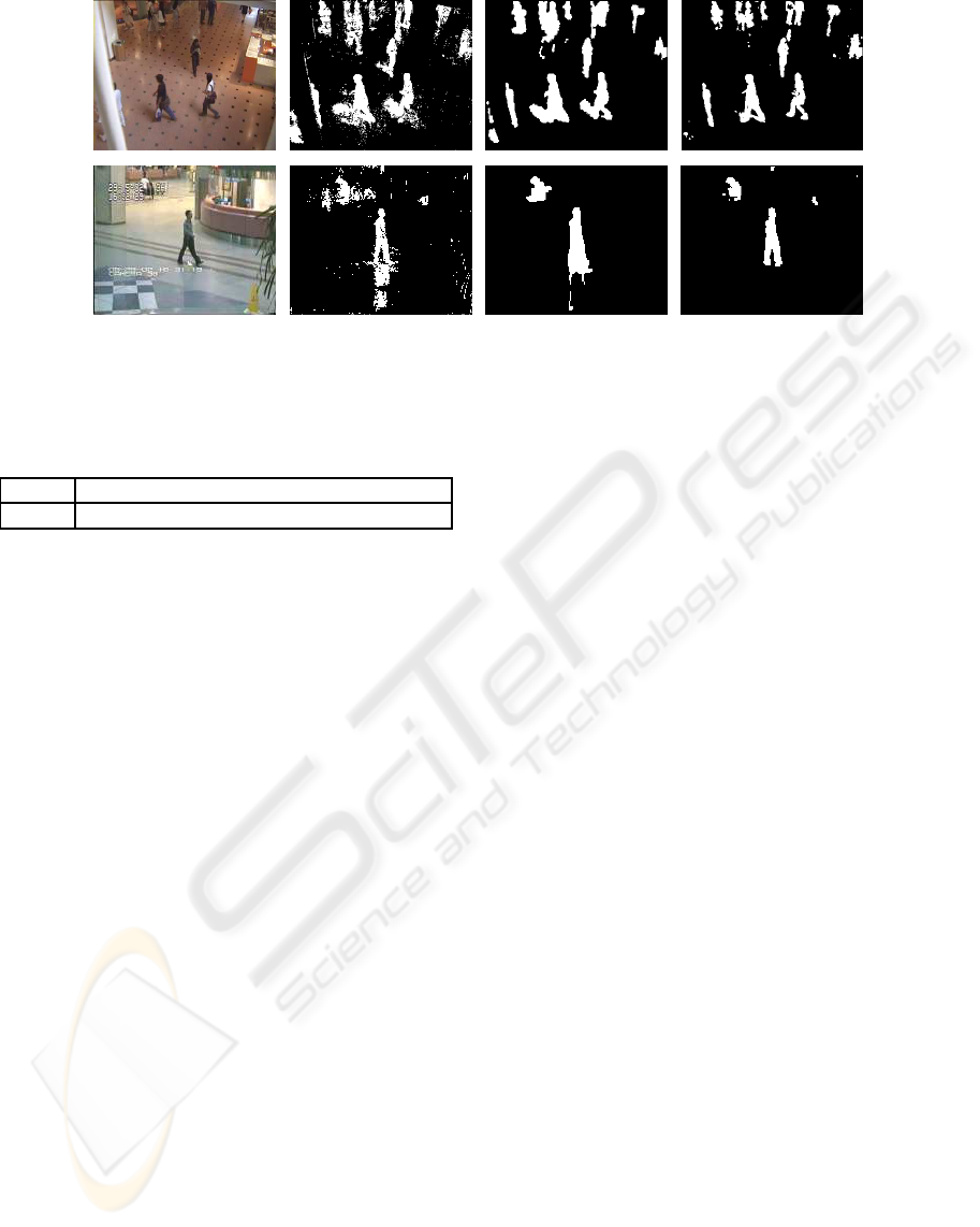
(a)
(b)
(c)
(d)
(a)
(b)
(c)
(d)
Figure 7: Original frame (a) and the corresponding detection results of the traditional method (b), the statistical background
modeling method (Li et al., 2004) (c) and the proposed method (d) for sequences Shopping (top) and Airport (bottom).
Table 4: Average detection frame rate for sequence Parking
using different numbers of threads.
threads 1 2 4 8 16 32
fps 29.20 48.54 60.16 73.21 75.43 72.76
ally expensive routines such as (Yang and Hsu, 2006).
Since the GMM estimation is done independently for
each pixel, parallel computing using multithreading
can further speed up the object detection process. Of
course it would not be practical to use a single thread
for each pixel. Thus, we devide each frame into n
slices. The slices are then parallel processed. By
using multithreading we increased the frame rate as
shown in Table 4. For each number of threads the
algorithm was run 100 times and the obtained frame
rates were then averaged.
5 CONCLUSIONS
A moving object detection method based on spatio-
temporal adaptive GMMs is proposed. The proposed
method significantly increases the quality of the de-
tection results without increasing the needed process-
ing time. Through parallelization of the algorithm we
further achievea speedup factor of up to 2.5 compared
to a single thread implementation.
ACKNOWLEDGEMENTS
The authors would like to thank Christoph Seeger for
his valuable assistance with the implementation of the
algorithm.
This work has been supported by the Gesellschaft
f¨ur Informatik, Automatisierung und Datenver-
arbeitung (iAd) and the Bundesministerium f¨ur
Wirtschaft und Technologie (BMWi), funding ID
20V0801I.
REFERENCES
Aach, T. and Kaup, A. (1995). Bayesian algorithms for
change detection in image sequences using Markov
random fields. Signal Processing: Image Communi-
cation, 7(2):147–160.
Carminati, L. and Benois-Pineau, J. (2005). Gaussian mix-
ture classification for moving object detection in video
surveillance environment. In Proc. IEEE Interna-
tional Conference on Image Processing, volume 3.
KaewTraKulPong, P. and Bowden, R. (2001). An im-
proved adaptive background mixture model for real-
time tracking with shadow detection. In Proc. 2nd
European Workshop Advanced Video Based Surveil-
lance Systems, volume 1.
Li, L., Huang, W., Gu, I., and Tian, Q. (2004). Statisti-
cal modeling of complex backgrounds for foreground
object detection. IEEE Transactions on Image Pro-
cessing, 13(11):1459–1472.
Porikli, F. and Tuzel, O. (2003). Human body tracking
by adaptive background models and mean-shift analy-
sis. In Proc. IEEE International Workshop on Perfor-
mance Evaluation of Tracking and Surveillance.
Power, P. W. and Schoonees, J. A. (2002). Understanding
background mixture models for foreground segmen-
tation. In Proc. Image and Vision Computing, pages
267–271.
Stauffer, C. and Grimson, W. E. L. (1999). Adaptive back-
ground mixture models for real-time tracking. In Proc.
IEEE Computer Society Conference on Computer Vi-
sion and Pattern Recognition, volume 2.
Yang, S. and Hsu, C. (2006). Background modeling from
gmm likelihood combined with spatial and color co-
herency. In Proc. IEEE International Conference on
Image Processing.
VISAPP 2010 - International Conference on Computer Vision Theory and Applications
418
