
VISUALIZATION OF UNCERTAIN CONTOUR TREES
Martin Kraus
Department of Architecture, Design, and Media Technology, Aalborg University
Niels Jernes Vej 14, DK-9220 Aalborg East, Denmark
Keywords:
Uncertainty visualization, Graph drawing, Information visualization, Volume visualization, Contour tree.
Abstract:
Contour trees can represent the topology of large volume data sets in a relatively compact, discrete data struc-
ture. However, the resulting trees often contain many thousands of nodes; thus, many graph drawing tech-
niques fail to produce satisfactory results. Therefore, several visualization methods were proposed recently
for the visualization of contour trees. Unfortunately, none of these techniques is able to handle uncertain con-
tour trees although any uncertainty of the volume data inevitably results in partially uncertain contour trees. In
this work, we visualize uncertain contour trees by combining the contour trees of two morphologically filtered
versions of a volume data set, which represent the range of uncertainty. These two contour trees are combined
and visualized within a single image such that a range of potential contour trees is represented by the resulting
visualization. Thus, potentially erroneous topological structures are visually distinguished from more certain
structures. Moreover, topological structures can be revealed that are otherwise obscured by data errors. We
present and discuss results obtained with a prototypical implementation using well-known volume data sets.
1 INTRODUCTION
Most of the topological structure of scalar volume
data sets can be efficiently represented by its contour
tree (Freeman and Morse, 1967), which is also a use-
ful data structure for several algorithms in volume vi-
sualization.
Unfortunately, contour trees of real volume data
sets tend to be extremely large even for small vol-
ume data sets (thousands or millions of nodes and
edges) since noise in the data results in many local
extrema and, therefore, in many nodes of the con-
tour tree. Thus, it is challenging to visualize contour
trees computed from real data. Moreover, most re-
searchers agree that one coordinate of the visualized
nodes should correspond to an isovalue in the volume
data set. With this requirement, however, it is impos-
sible to avoid crossing edges in the graph layout if
straight edges are employed.
In recent years, various techniques have been pro-
posed to visualize large contour trees of real volume
data sets using dot-and-line diagrams in two and three
dimensions with and without colors and/or icons.
Moreover, functions, surfaces, and terrains have been
proposed as well as combinations of stacked graphs
and Sankey diagrams.
However, the problem of uncertain volume data
has not been addressed by these approaches although
some uncertainty is usually inevitable, for example
because of measurements or simulations with finite
precision. Moreover, contour trees are susceptible
to arbitrarily small changes of the data of individ-
ual voxels, which can determine whether isosurface
components are separated or form a single compo-
nent, and therefore result in discrete changes of the
contour tree. The lack of visualization techniques for
uncertain contour trees is particularly remarkable as
uncertainty visualization for many other visualization
methods have been suggested in recent years and their
importance is widely accepted (Griethe and Schu-
mann, 2006; Johnson and Sanderson, 2003).
While some parts of contour trees are uncertain,
other parts may be stable against certain kinds of er-
rors and noise. One objective of this work is therefore
to propose a visualization of contour trees that con-
veys the difference between the uncertain parts of a
contour tree and its stable structures. Additionally,
our technique allows us to reveal further topological
structures, which might have been concealed by noise
or other data errors.
The data flow of the proposed technique is illus-
trated in Figure 1. Our approach is based on the obser-
vationthat the uncertainty of volume data corresponds
to the uncertain existence of components of isosur-
132
Kraus M. (2010).
VISUALIZATION OF UNCERTAIN CONTOUR TREES.
In Proceedings of the International Conference on Imaging Theory and Applications and International Conference on Information Visualization Theor y
and Applications, pages 132-139
DOI: 10.5220/0002817201320139
Copyright
c
SciTePress

volume data
@
@R
see Section 3
opened version
closed version
? ?
see (Kraus, 2010)
contour tree contour tree
@
@R
see Section 4
merged contour tree
with classified components
?
see Section 5
visualization
Figure 1: Data flow of the proposed technique.
faces and the uncertain separation between these com-
ponents. In order to detect uncertain components and
uncertain separations, we compute two versions of the
volume data set by means of grayscale morphology as
discussed in Section 3. To this end, we propose a new
variant of the opening operator that is capable of pre-
serving small components of isosurfaces.
While one of the two versions of the data set in-
cludes the stable components of isosurfaces, the sec-
ond version includes also uncertain and suspected
components. By computing contour trees for both
versions and matching their nodes, we can there-
fore determine which components and separations be-
tween components should be considered uncertain as
explained in Section 4. In order to visualize the result-
ing classification as described in Section 5, we extend
a recently proposed visualization of contour trees for
error-free data (Kraus, 2010).
The main contribution of this work is therefore the
use of grayscale morphology to determine the uncer-
tainty of the elements of a contour tree. In particular,
a new variant of the opening operator is suggested for
this purpose. Moreover, we show how to combine
multiple contour trees of different versions of a data
set in one visualization and how to visually convey
the uncertainty of their elements.
Results of a prototypical implementation of our al-
gorithm are presented in Section 6, while our conclu-
sions and plans for future work are discussed in Sec-
tion 7.
2 RELATED WORK
One of the first discussions of the contour tree
was published by Freeman and Morse (Freeman and
Morse, 1967). Efficient algorithms for the computa-
2 18 2845 84101 122 137 179 228
logarithmic surface area
isovalue
Figure 2: Visualization of the contour tree of the fuel data
set with markers for the 10 isosurfaces shown in Figure 3.
tion of contour trees were published, for example, by
Carr et al. (Carr et al., 2004) and Pascucci et al. (Pas-
cucci and Cole-McLaughlin, 2002; Pascucci et al.,
2004).
Visualizations of contour trees are often based on
dot-and-line diagrams in two dimensions (Bajaj et al.,
1997; Pascucci and Cole-McLaughlin, 2002; Carr
et al., 2004) or three dimensions (Takahashi et al.,
2004a; Takahashi et al., 2004b; Pascucci et al., 2004).
Furthermore, the use of icons has been proposed by
Shinagawa et al. (Shinagawa et al., 1991). As it is
difficult to match the resulting graph drawing to the
scalar field, the use of colors has been proposed to
identify connected components(Carr et al., 2004; We-
ber et al., 2007b; Weber et al., 2007a). Furthermore,
Weber et al. suggested the metaphor of a topological
landscape (Weber et al., 2007b). Note that all these
visualization techniques are limited to the visualiza-
tion of one error-free contour tree at a time.
In our work, contour trees are computed by the
method published by Kraus (Kraus, 2010), who also
presented a visualization technique for contour trees.
As depicted in Figure 2, contour trees are visualized
within a logarithmic plot of the area of isosurfaces
as a function of the corresponding isovalues. Alter-
natively, a histogram plot could also be employed.
This visualization can be considered a combination of
stacked graphs (see the works by Havre et al. (Havre
et al., 2002) and Byron and Wattenberg (Byron and
Wattenberg, 2008) and references therein) and Sankey
diagrams (Riehmann et al., 2005) or flow maps (Phan
et al., 2005). Related combinations of stacked bar
charts and Sankey diagrams were published by Fry
(Fry, 2004, section 4.6) and by Rosvall and Bergstrom
(Rosvall and Bergstrom, 2008). The approach is also
related to the representation of “levelset trees” as one-
dimensional functions by Klemel¨a (Klemel¨a, 2004),
although level set trees are not identical to contour
trees.
VISUALIZATION OF UNCERTAIN CONTOUR TREES
133
2 18 28 45 84 101 122 137 179 228
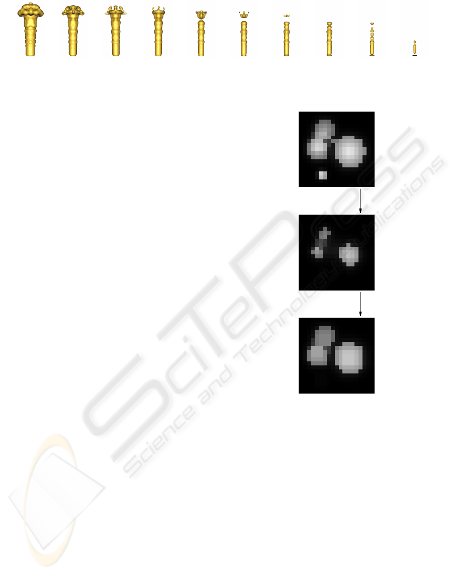
Figure 3: Isosurfaces of the fuel data set for the isovalues indicated in Figure 2.
In this work, we extend the approach of Kraus
to the case of uncertain contour trees by combining
the visualization of multiple contour trees in a single
image. Uncertainty visualization has been an estab-
lished topic in scientific visualization for several years
(Johnson and Sanderson, 2003). A survey of this re-
search was published by Griethe and Schumann (Gri-
ethe and Schumann, 2006). One of the most common
techniques to visualize uncertainty is the utilization of
free graphical variables, in particular color. However,
the simultaneous use of color to visualize data and its
uncertainty at the same time is problematic. For ex-
ample, Kardos et al. (Kardos et al., 2006) found that
the utilization of saturation to visualize uncertainty
is rather ineffective if hue is employed to visualize
the actual data. Differences between graphs are usu-
ally determined by graph matching techniques and are
also often visualized by color coding as discussed, for
example, by Delugach and de Moor (Delugach and
de Moor, 2005).
Grayscale morphology was published by Stern-
berg (Sternberg, 1986) and is a well-established im-
age processing technique, in particular for segmenta-
tion of medical data. In this context, grayscale mor-
phology is therefore more suitable to determine the
uncertainty of parts of the contour tree than simpli-
fication methods for contour trees, which were sug-
gested, for example, by Carr et al. (Carr et al., 2004)
and Pascucci et al. (Pascucci et al., 2004). Moreover,
grayscale morphology allows us to reveal additional
topological structures that might have been hidden by
data errors.
3 MORPHOLOGICAL IMAGE
PROCESSING
We employ opening and closing operators of
grayscale morphology (with a flat structuring func-
tion) to compute two versions of the data set, which
contain uncertain and certain topological structures,
respectively. The degree of uncertainty can be con-
trolled by the number of applications of these mor-
phological operators. In this work, however, we only
show results for at most one application of each oper-
ator.
original data
standard erosion
dilation
opened version
Figure 4: Illustration of a standard opening operation (ero-
sion followed by dilation).
3.1 Modified Opening
To reveal uncertain topological structures that are ob-
scured by noise, we apply a new variant of the open-
ing operator.
The standard opening is illustrated in Figure 4 and
starts with an erosion, which is applied to each voxel
v:
f
v
← min
w∈N(v)
{ f
w
}
where f
v
is the data value of voxel v and N(v) is the
set of the 26 neighbors of v and v itself. This erosion
is followed by a dilation:
f
v
← max
w∈N(v)
{ f
w
}
IVAPP 2010 - International Conference on Information Visualization Theory and Applications
134
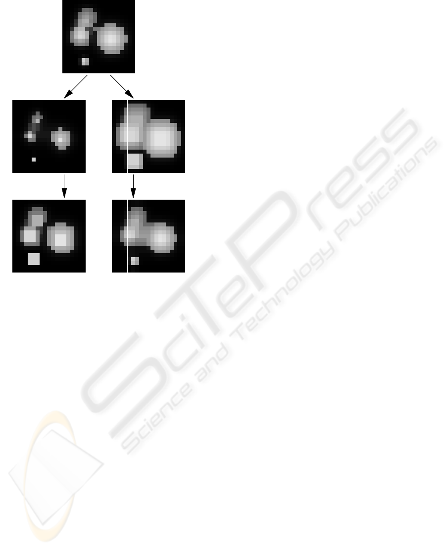
original data
modified erosion dilation
dilation erosion
opened version
with preserved maxima
closed version
Figure 5: Opening with preservation of maxima (left) and
closing (right).
Almost separated peaks and plateaus in the data set
will be separated by the opening operator. Addition-
ally, small separations tend to be widened. Thus, iso-
surface components are often split into multiple sepa-
rated components by the opening operator. In terms of
the contour tree, this corresponds to additional edges.
Therefore, topological structures that were obscured
by noise or other errors can be revealed by the open-
ing operator.
However, the standard opening operator also re-
moves peaks from the data as shown in Figure 4.
Since these peaks correspond to small isosurface
components, the opening can also prune edges from
the contour tree. There are several reasons why this
removal of edges is undesirable in the context of this
work. First of all, small isosurface components might
be removed by the standard opening operator and
joined with a nearby component by the closing op-
erator; thus, they vanish in both cases even though
they exist in the original data. This contradicts the
idea of representing the range of uncertainty by only
two versions of the data. Furthermore, the merging
and rendering of the two contour trees computed from
the opened and closed volumes can be significantly
simplified if the “closed tree” (the contour tree com-
puted from the closed data set) is a pruned version
of the “opened tree” (the contour tree computed from
the opened data set); i.e., if no edges of the latter are
removed.
Due to these considerations, we propose a new
variant of the opening operator that tries to preserve
arbitrarily small peaks. While the dilation is un-
changed, the modified erosion is:
f
v
←
f
v
if f
v
= max
w∈N(v)
{ f
w
}
min
w∈N(v)
{ f
w
} otherwise
This erosion operator is illustrated in Figure 5. It
makes sure that the data values of local maxima
are preserved by the corresponding opening operator.
While it might still remove some very small isosur-
face components, it cannot remove components that a
larger than about one voxel.
3.2 Closing
The standard closing consists of a dilation, i.e.,
f
v
← max
w∈N(v)
{ f
w
},
followed by an erosion, i.e.,
f
v
← min
w∈N(v)
{ f
w
}.
The closing joins peaks and plateaus that are close to
each other as illustrated in Figure 5. Thus, isosur-
face components are often joined and their total num-
ber is reduced. The remaining isosurface components
are therefore considered particularly stable or “cer-
tain.” In terms of the contour tree, this corresponds
to a pruning of the tree. In fact, our algorithm as-
sumes that the closed tree is a pruned version of the
opened tree. Therefore, it is unnecessary to preserve
local extrema in the way we proposed for the opening
operator.
3.3 Variants
By modifying the neighborhood N(v) or applying
the dilation and erosion operators multiple times, the
level of uncertainty can be adjusted to specific re-
quirements.
It should also be noted that the employed visual-
ization of the contour tree (Kraus, 2010) is a conser-
vative approximation in the sense that it never shows a
separation between two isosurface components unless
they are clearly separated in the volume data, i.e., only
rather stable components are visualized. If this kind
VISUALIZATION OF UNCERTAIN CONTOUR TREES
135

of conservative visualization is employed, the closing
might not be necessary but the original data can be
used instead.
4 MERGING MULTIPLE
CONTOUR TREES
After different versions of the original data set have
been compute by morphological image processing
(see Section 3), an approximation to the contour tree
is computed for each version of the data set as de-
scribed in (Kraus, 2010). Then, these contour trees
are merged into one tree and the uncertainty of their
nodes is determined.
While it is possible to merge any number of con-
tour trees, we will focus on the case of just two trees:
the “opened tree,” which is based on the morphologi-
cally opened data set, and the “closed tree,” which is
based on the morphologically closed data set. Fur-
thermore, we will assume that the closed tree is a
pruned version of the opened tree; i.e., it lacks some
(uncertain) nodes of the opened tree but it has no ad-
ditional nodes.
The approximate computation of the contour tree
described in (Kraus, 2010) partitions the whole data
range into uniform intervals. For each interval, it
determines the voxels with data values in the inter-
val and computes connected groups of these voxels,
which are used to approximateconnected components
of isosurfaces. These are the nodes of the computed
contour tree. Moreover, overlaps between connected
components of neighboring intervals are recorded in
order to construct edges of the contour tree.
In this work, we also record the largest overlap of
each connectedcomponent in the opened data set with
the connected components in the closed data set for
the same data interval. If no such overlap exists for a
specific connected component of the opened data set
then this component is removed from the processing.
The recorded overlaps allow us to match the nodes
of the two trees instead of matching their tree struc-
tures. Specifically, we distinguish the following cases
for each node of the closed tree:
1. No node of the opened tree is matched to a spe-
cific node of the closed tree: This contradicts our
assumption that the opened tree contains all nodes
of the closed tree. Nonetheless the node of the
closed tree is included in the merged tree since
this does not result in any ambiguities.
2. Exactly one node of the opened tree is matched
to the node of the closed tree: In this case the
two nodes are merged into one; in particular, all
recorded overlaps with nodes of neighboring data
intervals are inherited from the two nodes.
3. More than one node of the opened tree is matched
to the node of the closed tree: In this case,
the nodes of the opened tree are included in the
merged tree but the node of the closed tree is not.
Recorded overlaps with the latter node are ignored
since they are ambiguous.
Merging nodes consists mainly of merging the lists
of edges to other nodes of neighboring data intervals.
Moreover, references to merged nodes have to be ad-
justed. The main advantage of this approach is that
the resulting merged tree can be visualized in a simi-
lar way as described in (Kraus, 2010).
5 VISUALIZING MERGED
CONTOUR TREES
Our visualization of the merged contour tree is based
on a visualization technique for contour trees of error-
free data, which was presented in (Kraus, 2010). This
method computes x coordinates of the nodes based
on the data intervals of the corresponding connected
components. The y coordinates are computed by first
sorting the nodes of each data intervalin order to min-
imize the number of crossing edges, in particular of
edges that include at least one relatively large con-
nected component. Then, partial sums of the surface
area of the connected components are computed to
determine the actual y coordinates of the nodes.
The resulting grid of vertices is used to draw sep-
arating lines between nodes that are not connected
by edges, which correspond to recorded overlaps be-
tween connected components as discussed in Sec-
tion 4. More details and several examples of this vi-
sualization technique are presented in (Kraus, 2010).
In order to adapt this visualization to the merged
contour tree, we distinguish between separating lines
that mark uncertain structures and all others. To clas-
sify a separating line, the two connected components
that are separated by the line are considered. If they
are both part of the “opened tree” (see Section 4) and
the primary overlaps of both components refer to the
same connected component of the “closed tree” then
the separating line is considered uncertain since it is
an internal separation within the same certain compo-
nent of the closed tree.
It should be noted that arbitrarily many compo-
nents of the opened tree can be associated with a sin-
gle component of the closed tree. Moreover, these un-
certain separations can also extend over several data
intervals and thus form arbitrarily deep tree structures.
IVAPP 2010 - International Conference on Information Visualization Theory and Applications
136

Table 1: Timings for computing and rendering the visualizations in Figure 6. All visualizations decompose the data range into
200 intervals. The fuel data set and the silicium data set are trilinearly upsampled versions of the publicly available data sets
(Bartz, 2005; Levoy, 2001).
time in seconds
data set size original original + closed original + opened closed + opened
fuel 127× 127× 127 5 110 112 79
silicium 195 × 67× 67 16 188 219 197
CT head 256 × 256× 113 86 384 470 452
The lines between uncertain structures are ren-
dered in a different color than the other separating
lines. The former color should be closer to the back-
groundcolor in order to convey the idea of a weaker or
less certain separation. In this work, however, bright
red is used in order to emphasize these lines. Exam-
ples of the visualization are presented in the next sec-
tion.
6 RESULTS
We present results for three publicly available data
sets (Levoy, 2001; Bartz, 2005). Figure 6 shows a
comparison between the original contour tree visual-
ization (Kraus, 2010) for these data sets in the second
row and the proposed generalization of this visualiza-
tion in the third, fourth, and fifth row. The differences
between pairs of contour trees are marked by red lines
in order to emphasize them.
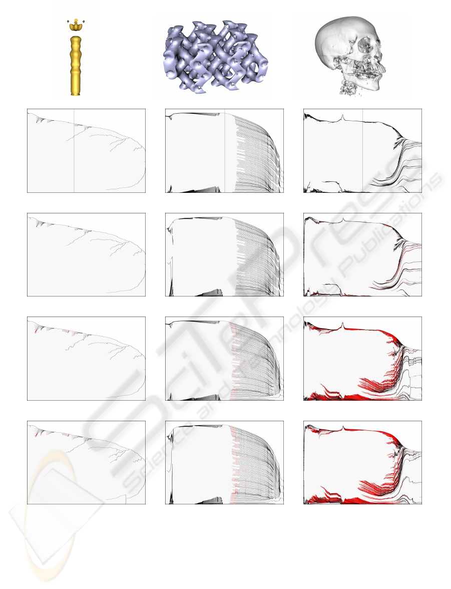
The third row depicts the differences between the
contour trees of the original data and the contour trees
of the morphologically closed data. Since the clos-
ing operation can join separated isosurface compo-
nents, some parts of the original separating lines are
no longer valid. These parts are marked in red in the
visualization. In most cases only the ends of the sep-
arating lines are affected. There are, however, also
some cases (in particular in complex data sets) where
a separation vanishes for all relevant isovalues. Since
a single closing operation will only join hardly sep-
arated components, the red lines indicate uncertain
separations.
In the fourth row the differences between the con-
tour trees of the original data and the contour trees of
the morphologically opened data is shown. The open-
ing operation can separate connected isosurface com-
ponents; thus, additional separating lines are intro-
duced, which are marked in red. These lines usually
extend lines of the original visualization to a larger
range of isovalues. However, there are also cases of
additional structures, which are only revealed by the
opening operation. The opening operation can sepa-
rate components, which are connected in the original
data. Thus, the additional separating lines are only
conjectured, i.e., they are less certain than the separa-
tions in the original visualization.
For the sake of completeness, the fifth row com-
bines the contour trees of the morphologically closed
and opened data set. Again, the differences are
marked in red.
Our prototypical implementation was tested on a
PC equipped with 2 GB RAM and two 3.6 GHz Pen-
tium 4 CPUs (only one was used to run the program).
Timings for the three data sets depicted in Figure 6
are summarized in Table 1. The computational costs
of merging two contour trees appear to be rather high;
however, no attempts have been made to optimize the
code.
7 CONCLUSIONS AND FUTURE
WORK
By employing grayscale morphology we can compute
multiple versions of a data set, which include either
more or less certain separations of isosurface com-
ponents than the original data set. Using these ver-
sions of the data, the proposed visualization of multi-
ple contour trees in a single image allows us to vi-
sually distinguish the more certain parts of a con-
tour tree from the less certain parts. Thus, it enables
us to visualize uncertain structures in contour trees.
Apart from this interpretation, our proposed visual-
ization can also be considered a preview of the effects
of grayscale morphological filters.
This work demonstrates that uncertainty visual-
ization is feasible even for very large graphs. We
achieved this goal by matching the objects repre-
sented by the nodes of two graphs (i.e., measuring the
overlap of isosurface components) instead of match-
ing the abstract structure of the two graphs, which
would introduce additional ambiguities and uncer-
tainties.
Future work includes performance optimizations,
the adjustment of the visualization to the actual de-
VISUALIZATION OF UNCERTAIN CONTOUR TREES
137
logarithmic surface area
isovalue
logarithmic surface area
isovalue
logarithmic surface area
isovalue
logarithmic surface area
isovalue
logarithmic surface area
isovalue
logarithmic surface area
isovalue
logarithmic surface area
isovalue
logarithmic surface area
isovalue
logarithmic surface area
isovalue
logarithmic surface area
isovalue
(a)
logarithmic surface area
isovalue
(b)
logarithmic surface area
isovalue
(c)
Figure 6: Visualizations of contour trees in plots of the logarithmic surface area for (a) the fuel data set, (b) the silicium
data set, and (c) the CT head data set. From top to bottom: an isosurface from the data set (first row), the standard contour
tree visualization with a vertical bar indicating the isovalue corresponding to the isosurface (second row), differences to the
morphologically closed data set marked in red (third row), differences to the morphologically opened data set marked in red
(fourth row), and differences between the closed and the opened data set marked in red (fifth row).
gree of uncertainty of the data, and the computation
and visualization of the degree of uncertainty. Further
plans include generalizations to different image pro-
cessing operations, and the integration of alternative
computations of contour trees.
IVAPP 2010 - International Conference on Information Visualization Theory and Applications
138

REFERENCES
Bajaj, C. L., Pascucci, V., and Schikore, D. R. (1997). The
contour spectrum. In Proceedings of the conference
on Visualization ’97, pages 167–ff.
Bartz, D. (2005). Volren and volvis homepage. URL:
http://www.volvis.org/; last accessed November 18,
2009.
Byron, L. and Wattenberg, M. (2008). Stacked graphs —
geometry & aesthetics. Visualization and Computer
Graphics, IEEE Transactions on, 14(6):1245–1252.
Carr, H., Snoeyink, J., and van de Panne, M. (2004). Simpli-
fying flexible isosurfaces using local geometric mea-
sures. In Proceedings of the conference on Visualiza-
tion ’04, pages 497–504.
Delugach, H. and de Moor, A. (2005). Difference graphs.
In Common Semantics for Sharing Knowledge: Con-
tributions to ICCS 2005. kassel university press.
Freeman, S. and Morse, S. P. (1967). On searching a con-
tour map for a given terrain elevation profile. Journal
of the Franklin Institute, 284(1):1–25.
Fry, B. J. (2004). Computational Information Design. PhD
thesis. Supervisor: John Maeda.
Griethe, H. and Schumann, H. (2006). The visualization of
uncertain data: Methods and problems. In Proceed-
ings of SimVis06, pages 143–156.
Havre, S., Hetzler, E., Whitney, P., and Nowell, L. (2002).
Themeriver: Visualizing thematic changes in large
document collections. Visualization and Computer
Graphics, IEEE Transactions on, 8(1):9–20.
Johnson, C. R. and Sanderson, A. R. (2003). A next step:
Visualizing errors and uncertainty. IEEE Computer
Graphics and Applications, 23(5):6–10.
Kardos, J., Moore, A., , and Benwell, G. (2006). Express-
ing attribute uncertainty in spatial data using blink-
ing regions. In Proceedings of the 7th International
Symposium on Spatial Accuracy Assessment in Natu-
ral Resssources and Environmental Sciences.
Klemel¨a, J. (2004). Visualization of multivariate density es-
timates with level set trees. Journal of Computational
and Graphical Statistics, 13(3):599–620.
Kraus, M. (2010). Visualizing contour trees within his-
tograms. In Proceedings of Computer Graphics and
Imaging (CGIM 2010). Accepted for publication.
Levoy, M. (2001). The stanford volume data archive.
URL: http://graphics.stanford.edu/data/voldata/; last
accessed November 18, 2009.
Pascucci, V. and Cole-McLaughlin, K. (2002). Efficient
computation of the topology of level sets. In Pro-
ceedings of the conference on Visualization ’02, pages
187–194.
Pascucci, V., Cole-McLaughlin, K., and Scorzelli, G.
(2004). Multi-resolution computation and presenta-
tion of contour trees. In Proceedings IASTED Confer-
ence Visualization, Imaging, and Image Processing,
pages 452–290.
Phan, D., Xiao, L., Yeh, R., Hanrahan, P., and Winograd,
T. (2005). Flow map layout. In Proceedings of the
2005 IEEE Symposium on Information Visualization,
page 29.
Riehmann, P., Hanfler, M., and Froehlich, B. (2005). Inter-
active Sankey diagrams. In Proceedings of 2005 IEEE
Symposium on Information Visualization, page 31.
Rosvall, M. and Bergstrom, C. T. (2008). Map-
ping change in large networks. URL:
http://arxiv.org/abs/0812.1242v1; last accessed
November 18, 2009.
Shinagawa, Y., Kunii, T., and Kergosien, Y. (1991). Sur-
face coding based on morse theory. IEEE Computer
Graphics and Applications, 11(5):66–78.
Sternberg, S. (1986). Grayscale morphology. Computer
Vision, Graphics, and Image Processing, 35(3):333–
355.
Takahashi, S., Takeshima, Y., and Fujishiro, I. (2004a).
Topological volume skeletonization and its applica-
tion to transfer function design. Graph. Models,
66(1):24–49.
Takahashi, S., Takeshima, Y., Nielson, G. M., and Fujishiro,
I. (2004b). Topological volume skeletonization using
adaptive tetrahedralization. Geometric Modeling and
Processing, 2004. Proceedings, pages 227–236.
Weber, G., Bremer, P.-T., and Pascucci, V. (2007a). Topo-
logical landscapes: A terrain metaphor for scientific
data. Visualization and Computer Graphics, IEEE
Transactions on, 13(6):1416–1423.
Weber, G. H., Dillard, S. E., Carr, H., Pascucci, V., and
Hamann, B. (2007b). Topology-controlled volume
rendering. Visualization and Computer Graphics,
IEEE Transactions on, 13(2):330–341.
VISUALIZATION OF UNCERTAIN CONTOUR TREES
139
