ESTIMATION OF CURVATURES IN POINT SETS BASED ON
GEOMETRIC ALGEBRA
Helmut Seibert
a
, Dietmar Hildenbrand
b
, Meike Becker
b
and Arjan Kuijper
a
a
Fraunhofer Institute for Computer Graphics Research, Darmstadt, Germany
b
Graphics Systems Group, Technical University of Darmstadt, Germany
Keywords:
Principal curvature, Curvature estimation, Geometric algebra, Point set.
Abstract: For applications like segmentation, feature extraction and classification of point sets it is essential to know the
principal curvatures and the corresponding principal directions. For the purpose of curvature estimation con-
formal geometric algebra promises to be a natural mathematical language: Local curvatures can be described
with the help of osculating circles or spheres. On one hand, conformal geometric algebra is able to directly
compute with these geometric objects, as well as with lines and planes needed for the description of vanishing
curvature. On the other hand, distance measures for fitting these objects into point sets can be handled in a
linear way, leading to efficient algorithms.
In this paper we use conformal geometric algebra advantageously in order to locally compute continuous
curvatures as well as principal curvatures of point sets without the need of costly pre-processing of raw data.
We show results on artificial and real data. Numerical verification on artificial data shows the accuracy of our
approach.
1 INTRODUCTION
The curvature of a surface is a feature which de-
scribes local surface properties in a well defined man-
ner. Each certain location has a minimal and a maxi-
mal principal curvature with orthogonal principal di-
rections. In (Alliez et al., 2003) this information
is used to obtain lines of curvature and umbilical
points as basis for a remeshing of surfaces. Other do-
mains are feature extraction for local comparison of
shapes (Gatzke et al., 2005), classification, registra-
tion or for instance the estimation of surface proper-
ties such as surface roughness (Lavoue, 2007) which
uses this measure for object segmentation. There-
fore, curvature estimation has become an important
topic of research (Kalogerakis et al., 2007; Yang et al.,
2006). Point set surfaces are verypopular in computer
graphics because they are powerful surface represen-
tations based on raw scanner data (Gross and Pfister,
2007), although it requires some effort to reconstruct
the surface from these (noisy) point clouds (Hornung
and Kobbelt, 2006; Mederos et al., 2005; Kolluri
et al., 2004; Mitra et al., 2004; Adamson and Alexa,
2003). As a consequence, computing curvatures from
point clouds without explicitly computing the surface
(-mesh) is extremely difficult. Approaches to tackle
this problem use statistics (Kalogerakis et al., 2007),
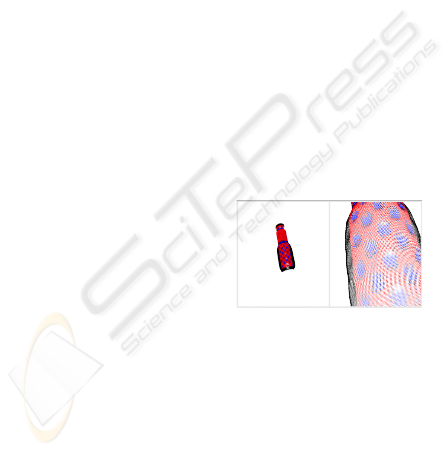
Figure 1: Point rendering of shape index estimated from
a point, the shown point-set is the raw output of a struc-
tured light reconstruction system without preprocessing like
smoothing or reduction. A pattern of concave areas and
some noise caused by the reconstruction process can be ob-
served at the surface of the bottle. The proposed algorithm
extracts the curvature on a local neighborhood yielding a
basis for object segmentation or feature detection.
or fitting of quadratic functions as local polynomial
(Gois et al., 2006). In order to determine local cur-
vature of point sets, we use the fitting of spheres.
This relates to the algebraic point set surfaces (Guen-
nebaud and Gross, 2007). We use conformal geo-
metric algebra, see e.g. (Vince, 2008) to describe
the local curvature of point sets because it allows to
treat geometric objects like spheres, circles, planes
and lines as easy as vectors in vector algebra. An-
12
Seibert H., Hildenbrand D., Becker M. and Kuijper A. (2010).
ESTIMATION OF CURVATURES IN POINT SETS BASED ON GEOMETRIC ALGEBRA.
In Proceedings of the International Conference on Computer Vision Theory and Applications, pages 12-19
DOI: 10.5220/0002817800120019
Copyright
c
 SciTePress

other reason is that it provides a linear distance mea-
sure between points and these geometric objects. Os-
culating circles describe the curvature of curves. The
local curvature of surfaces can be described with the
help of osculating spheres in all the tangent directions.
Spheres and circles, as well as lines and planes needed
for vanishing curvature, are handled very easily in
conformal geometric algebra. Its inner product gives
a linear measure between points and these geometric
objects. Therefore conformal geometric algebra, as a
5D extension of the 4D projective geometric algebra,
is a natural mathematical language to describe local
curvature of point sets.
The goal of this paper is to describe an algorithm
for the analysis of surface properties of scanned ob-
jects without the need of costly preprocessing of the
raw point set data. The main contributions of this pa-
per is to extend conformal geometric algebra meth-
ods in order to fit osculating circles (or lines) in dis-
crete tangent directions (see Section 3) and to com-
pute principal curvatures based on the estimation of
continuous curvaturesin all directions (see Section 4).
A first evaluation of the proposed algorithms and es-
timation results are given in Section 5.
2 RELATED WORK
The estimation of surface curvaturesbased on discrete
samples is sensitive to noise, as principal curvatures
are second-order derivatives of the surface. Previous
work in the area of surface curvature estimation cov-
ered tensor averaging using polygon edges and poly-
hedral mesh approximation methods. In (Hameiri and
Shimshoni, 2003) the methods proposed by (Chen
and Schmitt, 1992) and (Taubin, 1995) have been re-
visited and improved in order to overcome problems
better with noisy data, as provided by 3D reconstruc-
tion systems.
While Moving Least Squares (MLS) surfaces as
described in (Alexa et al., 2001) are using local plane
fits based on weighted least squares, our approach is
inspired by algebraic point set surfaces as introduced
in (Guennebaud and Gross, 2007). The authors de-
scribe a MLS surface based on algebraic sphere fit-
ting. Using spheres instead of planes for the local fit-
ting allows to easily compute mean curvatures. In our
approach explained in Sections 3 and 4, we
• use an extension of weighted least squares of
spheres in order to locally estimate osculating cir-
cles into point sets
• compute not only the mean curvature but continu-
ous curvatures in all tangent directions.
Table 1: List of some basic geometric primitives provided
by the 5D conformal geometric algebra. The bold charac-
ters represent 3D entities (x is a 3D point, n is a 3D normal
vector and x
2
is the scalar product of the 3D vector x). The
two additional basis vectors e
0
and e
∞
represent the origin
and infinity. The parameter r represents the radius of the
sphere and the parameter d represents the distance of the
plane to the origin.
entity representation
Point P = x+
1
2
x
2
e
∞
+ e
0
Sphere S = P −
1
2
r
2
e
∞
Plane π = n+ de
∞
Our new circle estimation algorithm based on confor-
mal geometric algebra introduced in Section 3 is in-
spired by (Hildenbrand, 2005). Fitting the best suit-
able object in a set of points, whether it is a sphere
or a plane, becomes a simple task if conformal geo-
metric algebra primitives are used. Note that this is
similar to automatically adjusting the parameter indi-
cating how much the sphere degenerates to a plane
in the fitting process of algebraic point set surfaces
as described in (Guennebaud et al., 2008). Since the
inner product of conformal geometric algebra can be
used as a measure for distance in a linear way, this ap-
plication can be solved very efficiently with the help
of the Eigenvectors of a 5 × 5 matrix. This is already
a fast solution for the fitting of spheres or planes. Our
new algorithm of Section 3 for the fitting of osculat-
ing circles further improves the efficiency of the fit-
ting algorithm to the computation of the Eigenvectors
of a 3× 3 matrix. In contrast to other approaches re-
lying on surface approximations we use features of
conformal geometric algebra to overcome limitations
observed at the transition between planar and spheri-
cal surfaces.
3 OSCULATING CIRCLE
FITTING USING GEOMETRIC
ALGEBRA
We use the conformal geometric algebra in order to
handle points, spheres and planes in a very intuitive
way. Table 1 gives an overview on some confor-
mal geometric algebra entities and their representa-
tions. The inner product of the vectors representing
point, sphere and plane results in a scalar and can be
used as a measure for the distances between them (see
(Hildenbrand, 2005)).
We use this distance measure for our new ap-
proach to fitting of circles or lines into a set of points.
Let {p
i
∈ R
3
|i = 1, . . . , n} denote our point
cloud. The corresponding points in conformal geo-
ESTIMATION OF CURVATURES IN POINT SETS BASED ON GEOMETRIC ALGEBRA
13

metric algebra are then represented by
P
i
= p
i
+
1
2
p
2
i
e
∞
+ e
0
.
We assume that the points to be approximated are
roughly aligned in the direction of a tangent vector
at x (see Figure 2). Therefore our fitting task can be
reduced to the task of fitting a circle (or in the limit
case a line) in the direction of the normal vector. This
circle is also called the osculating circle in x. Let n be
the normal vector at the location x = (x
1
,x
2
,x
3
).
Figure 2: Estimation of curvature at x based on the fitting
of a sphere (or plane) with center point in the opposite di-
rection of the normal n into a set of points.
A sphere or plane K in conformal geometric alge-
bra is in general represented by the 5D vector
K = s
1
e
1
+ s
2
e
2
+ s
3
e
3
+ s
4
e
∞
+ s
5
e
0
,
for s
1
,...,s
5
∈ R.
If s
5
= 0 we get a plane, in the other case a sphere.
As described above we have given that the center of
the sphere S that we fit into our point set is m= x+rn,
where r ∈ R denotes the radius of the sphere. There-
fore we can represent the sphere as
S
′
= m+
1
2
(m
2
− r
2
)e
∞
+ e
0
.
Now we scale this sphere by t
3
∈ R and we get an
object of the form Equation 3 which can be a sphere
or a plane:
S = t
3
(m+
1
2
(m
2
− r
2
)e
∞
+ e
0
)
= t
3
m+t
3
e
0
+ t
2
e
∞
,
where t
2
=
1
2
t
3
(m
2
− r
2
).
The inner product of S and P
i
gives us a measure
for their distance:
P
i
· S = (p
i
+
1
2
p
i
2
e
∞
+ e
0
) · (t
3
(x+ rn) +t
3
e
0
+ t
2
e
∞
)
= t
1
(p
i
· n) − t
2
+ (p
i
· x−
1
2
p
i
2
)t
3
=
3
∑
j=1
w
ij
t
j
,
where t
1
= t
3
r and
w
ij
=





p
i
· n, j = 1
−1, j = 2
p
i
· x−
1
2
p
i
2
, j = 3.
(1)
In order to fit the best approximating sphere or
plane into the point set, we consider min
∑
n
i=1
(P
i
· S)
2
as residual for our least squares approach. Equiva-
lently, we can write the problem using the bi-linear
form as min
t∈R
3
(t
T
Bt), where t = (t
1
,t
2
,t
3
) and B is a
3× 3 matrix with entries
b
jk
=
n
∑
i=1
w
ij
· w
ik
, for j, k = 1, 2,3.
B is symmetric and we consider only normalized re-
sults t with t
T
t = 1, the given problem can be con-
sidered as an eigenvector problem and the solution is
given by the eigenvector corresponding to the small-
est eigenvalue of B.
4 PRINCIPAL CURVATURE
ESTIMATION
The idea of the proposed algorithm is as follows: A
discrete sampling of the surface curvature can be used
to obtain an estimation of the principal curvatures and
the corresponding principal directions.
An outline of the algorithm is as follows:
1. Local point selection with chosen estimation ra-
dius d
max
2. Local tangent frame definition
3. Define planes for n directions and select the points
closer than a chosen threshold t to each plane
4. Fitting of circles to the points for each direction
5. Estimate parameters for the curvature model func-
tion
6. Derive curvature information from model param-
eters
To evaluate the curvature of a surface represented as a
set S = {p
0
...p
n
} of points p
i
= (x
i
,y
i
,z
i
) at a certain
location x ∈ S, the set N = {p
i
∈ S | |x − p
i
| ≤ d
max
}
of neighboring points within a givendistance d
max
has
to be considered. To optimize the point selection ap-
propriate hierarchical representations of the surface S
such as octree or kd-tree can be used. Given addi-
tional information on the surface topology such as the
triangle indices, the k-ring neighbor method may be
suitable to access the neighborhood while reducing
the number of distance tests in point selection.
VISAPP 2010 - International Conference on Computer Vision Theory and Applications
14

The subsequent processing steps are applied with
respect to the tangent plane at point x. If the normal
n is not known a normal vector can be estimated by
applying a sphere/plane fit to the selected points, re-
sulting in a surface normal or a vector to the center
of an estimated sphere which can be normalized and
interpreted as a normal vector. In this case the ori-
entation of the surface is not defined from the local
perspective, additional effort by means of global sur-
face inspection is required. Given a normal vector n
an arbitrary point on the tangent plane can be used to
create one orthogonal basis vector t
u
. The second ba-
sis vector t
v
can be calculated using the cross product
t
v
= n× t
u
to define a local tangent frame.
To obtain a discrete sampling of the surface prop-
erties depending on the direction a set of n planes
perpendicular to the tangent plane has to be defined.
The normal l
i
for plane L
i
,i ∈ {1...n} can be cal-
culated by rotating the local tangent vector t
v
coun-
terclockwise around n by α
i
=
(i−1)·π
n
radians. As
all planes need to pass the reference point x, each
of the n planes L
i
can be defined in hessian nor-
mal form as (l
i
· n) − |x| = 0. For each plane L
i
the points p
j
within the neighborhood N whose dis-
tance to the plane is less than a predefined thresh-
old distance d
max
are collected into point sets D
i
=

p
j
∈ N | |(l
i
· n) − p
j
| ≤ d
max

, Figure 3 shows the
selected points within a chosen estimation radius. The
point sets D
i
are split into two segments each using
the plane L
i
rotated around the surface normal at x by
π
2
radians in order to perform the following fitting al-
gorithms on a larger set of samples coveringthe whole
revolution. Performing this operation allows to cap-
ture local discontinuities as present at edges as well.
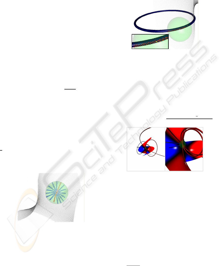
Figure 3: The selected point sets for 8 directions within es-
timation radius on a saddle surface are shown highlighted.
The curvature κ at the point x equals the inverse ra-
dius r of the osculating circle. The osculating circle
is estimated in a least squares sense by applying the
curve fit explained in Section 3. For each set of cross
section points D
i
a circle fit f
i
has to be performed.
The points p
j
∈ D
i
have been selected with respect to
the plane L
i
and the reference point x, the points p
j
represent the cross section of the originating surface
S with the plane. The fitting result for one direction
is illustrated in Figure 4, the results for a 8 direction
estimation can be seen in Figure 5.
Figure 4: Circle fitting result for one direction. The high-
lighted points within the estimation radius have been used
to approximate a circle. The resulting osculating circle is
visualized as a torus.
If the point sets D
i
have been split as mentioned above
the fitting has to be applied for each subset to obtain a
curvature sample. According to the Euler formula the
curvature values c(α) in direction of a tangent vector
t rotated around the reference point x with angle α
are defined as κ(α) = κ
1
· cos
2
(α) + κ
2
· sin
2
(α) with
the principal curvatures κ
1
and κ
2
, which can be rear-
ranged to the form κ(α) =
−(κ
1
−κ
2
)·sin(2α−
π
2
)+κ
1
+κ
2
2
.
Figure 5: The circle fitting results in a set of circles, each
shown as a torus for a certain direction. The base Surface
is a monkey saddle surface, the colors of the surface encode
the shape index. The osculating circles visualized as tori are
sized and oriented according to the directional estimation
results.
With κ
1
and κ
2
fixed it provides the simple model
for this function κ(α) = a · sin(α + ϕ) + o. This
model function is fitted to the sampled curvatures
by optimizing the amplitude a, phase ϕ and offset
o using the three parameter sine fit method (IEEE,
2001), which allows to obtain a least squares solution
r = (r
1
,r
2
,r
3
)
T
=

M
T
M

−1
·

M
T
f

with matrix M
defined appropriately using the angles α
i
and vector
f = ( f
1
, f
2
,··· , f
n
)
T
, which consists of the measured
curvatures. The result r can be converted to amplitude
a =
q
r
2
1
+ r
2
2
, phase
ESTIMATION OF CURVATURES IN POINT SETS BASED ON GEOMETRIC ALGEBRA
15

ϕ =



arctan

−
r
2
r
1
+
π
2

if r
1
> 0
arctan

−
r
2
r
1
+
3π
2

if r
1
< 0
and offset o = r
3
.
The maximum and minimum values of the model
function directly yield the maximum and minimum
curvature. The corresponding alignment of the prin-
cipal directions can be calculated using the angle of
minimum and maximum relative to the tangent frame
considering a phase correction ϕ to obtain angles of
the extrema κ
1/2
= a ± o:
v
max
=

sin

−ϕ+
π
2

,cos

−ϕ+
π
2

,0

v
min
=

sin

−ϕ+
3π
2

,cos

−ϕ+
3π
2

,0

The result of such an optimization for 16 samples
is shown in Figure 6.
-0.3
-0.25
-0.2
-0.15
-0.1
-0.05
0
0.05
0.1
0.15
22.5 45 67.5 90 112.5 135 157.5 180 202.5 225 247.5 270 292.5 315 337.5 360
curvature
phi
samples
fitting result
Figure 6: Sine fitting results. The curvature has been sam-
pled in 8 directions resulting in 16 measurements. The
sine function approximates the real distribution of curva-
tures yielding the location of curvature maxima and min-
ima and the corresponding direction angles with respect to
the local reference frame.
-0.3
-0.25
-0.2
-0.15
-0.1
-0.05
0
0.05
0.1
0.15
22.5 45 67.5 90 112.5 135 157.5 180 202.5 225 247.5 270 292.5 315 337.5 360
curvature
phi
samples
first fitting
second fitting
result
Figure 7: Refined fitting using a second model function with
half frequency. The sum of both model functions shows a
better approximation of the measured curvature samples.
As the curvature samples are present for each di-
rection, the samples cover two phases of the model
function. Curvature measurements for opposite direc-
tions differ, if curvature gradients are present. This al-
lows a second optimization, which uses the difference
between the sample value and the parametrized model
function to perform a second fitting of a sine function
with half frequency yielding amplitude a
2
, phase ϕ
2
and offset o
2
. The evaluation of this model function
at the location of maxima and minima can be used
to correct the curvature measurements and to derive
the direction of the gradient in the principal direction,
see Figure 7. The complete model function is then
c(α) = a·sin(α+ ϕ) +o+ a
2
·sin(0.5· α+ ϕ
2
) + o
2
.
The phase shift which may be introduced by this sum-
mation is usually small and has been ignored. The
maxima and minima derived by the first fitting have
been corrected choosing the lowest minimum value
and the highest maximum value. The vectors v
max
and v
max
are the principal curvature directions with
respect to the tangent frame. The local tangent frame
is defined by the three basis vectors t
u
, t
v
and n. The
rotation of the local tangent frame with respect to the
global object coordinate system is denoted R
tangent
global
.
The principal directions in object space can be calcu-
lated by applying inverse tangent rotation R
global
tangent
=
(R
tangent
global
)
−1
. The result is then p
max
= R
global
tangent
· v
max
and p
min
= R
global
tangent
· v
min
. The robustness and quality
of the model function fit can be increased using an
outlier detection and removal. This applies mostly to
irregular sampled and distorted surfaces. Choice and
evaluation of an appropriate method is subject to fur-
ther improvement of this approach.
4.1 Parameters and Suitable Ranges
The proposed algorithmic approach is controlled by
a set of parameters. The estimation radius defines
the size of the surface portion for the evaluation. The
estimation radius must be chosen considering two as-
pects. On the one hand it is necessary to select enough
points for the circle fitting and on the other hand it
must correspond to the maximum and minimum fea-
ture size to be detected. The number of estimation
directions respective of normal sections used for the
curvature estimation should be chosen small in order
to limit the computational effort and it should be big
enough to allow a reliable fitting of the model func-
tion. A choice of 8 estimation directions resulting in
16 samples provided a reasonable ratio of robustness
and accuracy for the performed tests.
The maximum plane distance for point selec-
tion defines the focus of the point selection with re-
spect to the plane, can be very small for high point
densities. Bigger values may decrease the estimation
quality as the optimal point set for circle estimation
would be coplanar. Concerning the parameters con-
trolling the point selection a choice must assure that
VISAPP 2010 - International Conference on Computer Vision Theory and Applications
16

there are enough points for the circle estimation al-
gorithm. A theoretical limit of three points must be
exceeded, while large amounts of points can be han-
dled without problems. In practice a point count be-
tween 10 and 30 for each circle estimation yielded
best results. Given special surface constellations as
closely located opposite surface areas within concave
surface regions this can only be identified if topologi-
cal information is present e.g. in triangle mesh struc-
tures. The estimation radius and the evaluation dis-
tance d
max
must be chosen carefully in order to detect
small features and to avoid topological misinterpreta-
tions. As the approach is suitable for dense sampled
surfaces or non optimized triangulated surfaces the
recommendation is to choose the radius as big as pos-
sible while being small with respect to the depicted
object structures.
5 RESULTS
The proposed algorithm has been evaluated consider-
ing the two basic optimization steps and the overall
performance. As the circle fit algorithm is intended to
be used on data acquired from the real world, several
properties of point sampled surface data have been
simulated in order to evaluatethe algorithm. The most
important influences are point density, point distribu-
tion, distortion and a range of radii are included in
the data generation process. The tests have been done
using points on a circle segment simulating a fixed
estimation window of width 4. According to each
performed test the radius, the number of points and
amount of noise have been varied. The noise has been
generated using a gaussian distribution and a fixed
level, as this is in practice introduced by the acqui-
sition process and should depend only on the distance
and viewing angles but not on the size and shape of
the surface.
As the estimation window size remains the same
for all radii it can be expected that estimation er-
rors grow with growing radii and growing amount of
noise. An optimal estimation algorithm would yield
the radius used for the point generation as estima-
tion result. The resulting radii are used within our
approach to determine the curvature, which is the re-
ciprocal value, e.g. the interpretation of the results
must take into account that errors occurring at the es-
timation of big radii result in smaller errors for low
curvature values, e.g. flat portions of the investigated
surface. An extension of the fitting algorithm to a
weighted least squares approach has been very in-
vestigated, too, but the results did not turn out to be
promising so far.
As the sampling density of 3D reconstruction data
is varying with respect to the measurement angle and
the measurement distance, one cannot always assume
regular distribution of the point samples. In these tests
12 points have been generated for some radii within
1 and 10000 using a regular angle dependent distri-
bution of points along the circle segment or a ran-
dom distribution. A normal distributed distortion with
σ = 0.5 has been added to investigate the influence of
noisy data. The test result is shown in Figure 8, with-
out noise the type of point distribution did not show
a significant influence. With an increasing amount of
noise the estimation quality decreased.In the observed
cases the distribution of points did not show a signif-
icant influence, while the circle fit algorithm tends to
overestimate the radii.
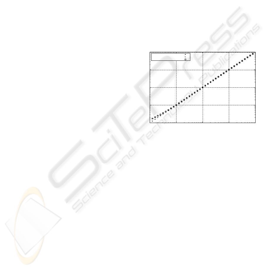
1
10
100
1000
10000
1 10 100 1000 10000
estimated radius
radius
GA circle fit random distributon vs. regular distribution
noise 0.0 - regular
noise 0.5 - regular
noise 0.5 - random
Figure 8: Circle fitting results for a regular and random re-
spectively distribution of 12 points on small segments of
circles with a fixed angle and increasing radii considering
distortion. The real radii are shown on the abscissa and the
estimated radii are on the ordinate. Without distortion an
optimal estimation can be observed resulting in a straight
line. In case of distortion the algorithm tends to overesti-
mate radii. In case of the regular point distribution a slightly
increased overestimation can be observed.
The next test shows the influence of the point
count on the estimation quality. The points are ran-
domly distributed, and the tested point counts were
4, 12 and 24. To point out the limits of the algo-
rithm a random point distribution and a gaussian noise
(σ = 0.5) have been chosen for this test. The esti-
mation errors observed are bigger at very small radii,
e.g. for bigger radii a quiet good estimation can be
achieved. Using a small point count of 4, the estima-
tion yields smaller radii than the real ones, while in-
creasing point counts of 24 yield slightly bigger radii.
In this test the point count of 12 showed the best esti-
mation result, see Figure 9. The estimation results for
all point counts without noise were optimal indepen-
dent of random or regular point distribution.
The sine fitting algorithm explained in Section
ESTIMATION OF CURVATURES IN POINT SETS BASED ON GEOMETRIC ALGEBRA
17

1
10
100
1000
10000
1 10 100 1000 10000
estimated radius
radius
GA circle fit number with different numbers of points
4 points
12 points
24 points
linear
Figure 9: Circle fitting results with respect to the number
of points. The increasing radii have been estimated using
different numbers of points considering a gaussian noise
(σ = 0.5).
4 has been evaluated choosing a certain amplitude,
phase and offset. For the chosen parameters several
samples with different levels of noise have been gen-
erated. The RMS error for the given samples with
respect to the estimated function has been observed
for an amount of four up to a hundred points. The
estimation results remain within the expected range
for all tested numbers of points. We assume that the
number of estimation directions does not have a sig-
nificant influence on the fitting quality, but the quality
of the samples heavily influences the results.
0
0.005
0.01
0.015
0.02
0.025
0 10 20 30 40 50 60 70 80 90 100
rms error
points
sine fit error with respect to point count
no noise
2.5% noise
5% noise
Figure 10: RMS Errors of the sine fitting algorithm used
for the fitting of the model function. The results are shown
for different sample counts, considering distortions of the
samples as well.
The proposed approach relies on two subsequent steps
of least-squares optimizations, each of which intro-
duce small errors. The achievable overall perfor-
mance is not yet comparable to the quiet exact evalua-
tion considering over the years optimized state-of the
art algorithms originating from the tensor method in-
troduced by Taubin (Taubin, 1995). Nevertheless, the
approach is efficient and robust to many aspects and
may be very useful to obtain an initial rough estima-
tion in large datasets.
Table 2: Surface curvature evaluation results for regions of
the saddle surface z = 0.2x
2
+0.1y
2
have been compared to
the known analytical values of the generating function. ∆κ
1
and ∆κ
2
denote the absolute value of the difference.
Point distrib. regular random
est. radius 2 2
est. directions 8 8
points 13926 14049
x min -10 -10
x max 10 10
∆ x 0.11 random
y min -10 -10
y max 10 10
∆ y 0.11 random
∆κ
1
min 0.000 0.000
∆κ
1
max 0.028 0.030
∆κ
1
mean 0.008 0.008
∆κ
1
stdd. 0.006 0.006
∆κ
2
min 0.000 0.000
∆κ
2
max 0.085 0.090
∆κ
2
mean 0.019 0.018
∆κ
2
stdd. 0.018 0.018
The results of the proposed algorithm have been
evaluated on basis of surfaces generated by simple bi-
variate functions. The real principal curvatures and
directions of these generator functions can be anal-
ysed exactly using the fundamental forms based on
the first and second derivatives. For each test a certain
range in the parameter space of the generator func-
tion has been chosen and theoretical curvature val-
ues and surface points have been compared to estima-
tions based on the proposed approach.The results are
shown in table 2. An example for the result of the pro-
posed approach applied to a real 3D reconstruction of
a small bottle is shown in Figure 1. The reconstructed
surface has some distortions caused by reflections of
the original bottle during acquisition. Nevertheless,
the estimated shape index allows an interpretation of
the surface structure.
The proposed methods provide several aspects we
would like to investigate in future work. The sam-
pling of curvatures in opposite directions from the
point may be used to exploit the curvature gradient
or to detect local discontinuities such as edges.
A first approach by setting up a model function
summing two sine functions with the first function
having the double frequency has been done. The
model function has been fitted using a linear sine fit-
ting approach. We are planning to explore different
optimization techniques like Levenberg-Marquardt
using a more complex model function. We assume
that dynamic sampling and rendering of point set sur-
faces can be improved by this method.
VISAPP 2010 - International Conference on Computer Vision Theory and Applications
18

6 CONCLUSIONS
In this paper we used geometric algebra techniques in
order to compute principal curvatures of point sets in
an elegant and efficient way. We could benefit espe-
cially from the property of geometric algebra of nat-
urally describing curvatures. On the one hand, geo-
metric algebra can easily describe geometric objects
like spheres and planes, circles and lines as well as
the limit between them. On the other hand its in-
ner product provides possibilities for a fast measure-
ment of distances. In a nutshell, we presented a novel
simple and efficient approach, which allows to access
curvature information within dense point sets without
costly preprocessing.
REFERENCES
Adamson, A. and Alexa, M. (2003). Approximating and
Intersecting Surfaces from Points . In Eurograph-
ics Symposium on Geometry Processing (SGP), pages
230–239.
Alexa, M., Behr, J., Cohen-Or, D., Fleishman, S., Levin,
D., and Silva, C. T. (2001). Point set surfaces. In
Conference on Visualization (VIS), pages 21–28.
Alliez, P., Cohen-Steiner, D., Devillers, O., L´evy, B., and
Desbrun, M. (2003). Anisotropic polygonal remesh-
ing. ACM Transactions on Graphics, 22(3):485–493.
Chen, X. and Schmitt, F. (1992). Intrinsic surface prop-
erties from surface triangulation. In European Con-
ference on Computer Vision (ECCV), pages 739–743,
London, UK. Springer-Verlag.
Gatzke, T., Grimm, C., Garland, M., and Zelinka, S. (2005).
Curvature Maps For Local Shape Comparison. In
Shape Modeling and Applications, pages 244–253.
Gois, J., Tejada, E., Etiene, T., Nonato, L., Castelo, A.,
and Ertl, T. (2006). Curvature-driven modeling and
rendering of point-based surfaces. In Brazilian Sym-
posium on Computer Graphics and Image Processing
(SIBGRAPI), pages 27–36.
Gross, M. and Pfister, H. (2007). Point Based Graphics.
Morgan Kaufmann.
Guennebaud, G., Germann, M., and Gross, M. (2008). Dy-
namic sampling and rendering of algebraic point set
surfaces. In Eurographics, pages 653–662.
Guennebaud, G. and Gross, M. H. (2007). Algebraic
point set surfaces. ACM Transactions on Graphics,
26(3):23.
Hameiri, E. and Shimshoni, I. (2003). Estimating the prin-
cipal curvatures and the darboux frame from real 3-d
range data. IEEE Systems, Man, and Cybernetics B
(SMC-B), 33(4):626–637.
Hildenbrand, D. (2005). Geometric computing in computer
graphics using conformal geometric algebra. Comput-
ers & Graphics, 29(5):802–810.
Hornung, A. and Kobbelt, L. (2006). Robust Reconstruc-
tion of Watertight 3D Models from Non-uniformly
Sampled Point Clouds Without Normal Information .
In Eurographics Symposium on Geometry Processing
(SGP), pages 41–50.
IEEE (2001). Std. 1241-2000 IEEE standard for terminol-
ogy and test methods foranalog-to-digital converters,
chapter 3, pages 26–27.
Kalogerakis, E., Simari, P., Nowrouzezahrai, D., and Singh,
K. (2007). Robust Statistical Estimation of Curvature
on Discretized Surfaces. In Eurographics Symposium
on Geometry Processing (SGP), pages 13–22.
Kolluri, R., Shewchuk, J. R., and O’Brien, J. F. (2004).
Spectral Surface Reconstruction From Noisy Point
Clouds . In Eurographics Symposium on Geometry
Processing (SGP), pages 11–22.
Lavoue, G. (2007). A Roughness Measure for 3D Mesh
Visual Masking. In ACM SIGGRAPH Symposium
on Applied Perception in Graphics and Visualization
(APGV), pages 57 – 60.
Mederos, B., Amenta, N., Velho, L., and de Figueiredo,
L. H. (2005). Surface Reconstruction for Noisy Point
Clouds. In Eurographics Symposium on Geometry
Processing (SGP), pages 53–62.
Mitra, N. J., Gelfand, N., Pottmann, H., and Guibas, L.
(2004). Registration of Point Cloud Data from a Ge-
ometric Optimization Perspective . In Symposium on
Geometry Processing, pages 23–32.
Taubin, G. (1995). Estimating the Tensor of Curvature of
a Surface from a Polyhedral Approximation. In IEEE
International Conference on Computer Vision (ICCV),
pages 902–907.
Vince, J. (2008). Geometric Algebra for Computer Graph-
ics. Springer.
Yang, Y.-L., Lai, Y.-K., Hu, S.-M., and Pottmann, H.
(2006). Robust Principal Curvatures on Multiple
Scales. In Eurographics Symposium on Geometry
Processing (SGP), pages 223–226.
ESTIMATION OF CURVATURES IN POINT SETS BASED ON GEOMETRIC ALGEBRA
19