DIRECT SURFACE FITTING
Nils Einecke, Sven Rebhan, Julian Eggert
Honda Research Institute Europe, Carl-Legien-Strasse 30, 63073 Offenbach, Germany
Volker Willert
Control Theory and Robotics Lab, TU Darmstadt, Landgraf-Georg-Strasse 4, 64283 Darmstadt, Germany
Keywords:
Stereo, Model fitting, Surface estimation, 3-D perception.
Abstract:
In this paper, we propose a new method for estimating the shape of a surface from visual input. Assuming a
parametric model of a surface, the parameters best explaining the perspective changes of the surface between
different views are estimated. This is in contrast to the usual approach of fitting a model into a 3-D point cloud,
generated by some previously calculated local correspondence matching method. The main ingredients of our
approach are formulas for a perspective mapping of parametric 3-D surface models between different camera
views. Model parameters are estimated using the Hooke-Jeeves optimization method, which works without
the derivative of the objective function. We demonstrate our approach with models of a plane, a sphere and a
cylinder and show that the parameters are accurately estimated.
1 INTRODUCTION
A basic step of many stereo algorithms is the compu-
tation of a disparity or depth map by means of a local
correspondence search. Instead of comparing single
pixels a local window around each pixel is used be-
cause pixel comparisons are prone to produce false
correspondences. This constitutes a local smooth-
ness assumption, which dramatically improvesthe de-
tected correspondences. However, some correspon-
dences are still wrong due to repetitive patterns, cam-
era noise or slight view changes between different
camera images. In order to remove such erroneous
correspondences and to improve the accuracy, more
global smoothness assumptions are applied to the re-
sulting disparity maps. A common way of doing so,
is to fit basic surface models, e.g. planes (Bleyer
and Gelautz, 2005; Hirschm¨uller, 2006; Klaus et al.,
2006; Wang and Zheng, 2008), into the 3-D point data
that can be extracted from the disparity maps.
In this paper, we present an alternative approach
which integrates parametric surface models directly
into the correspondence search. This means that we
fit surface models directly to the image data and not
into some preprocessed disparity maps. This leads to
a much higher accuracy because the original stereo
input images carry the complete visual information
while the disparity maps contain only the extracted
depth information. Furthermore, the model-based
correspondence search allows to estimate the depth
for large image regions at once, which also improves
robustness and accuracy. The basic idea of our ap-
proach is to estimate depth by means of the perspec-
tive view changes a surface undergoes between dif-
ferent camera views. To achieve this, we describe
the perspective view changes of a surface via its para-
metric description, e.g. center and radius of a sphere
or anchor point and rotation angles of a plane. The
parameters of a surface model are estimated using
Hooke-Jeeves (Hooke and Jeeves, 1961) optimiza-
tion, which is a direct search method. Its objective
is to find those parameters which explain the perspec-
tive view changes best.
Early work on incorporating models of the 3-D
scene geometry directly into the correspondence
search was done by Cernuschi-Frias et al. (Cernuschi-
Frias et al., 1989). The authors presented a framework
for estimating parameters of different surface mod-
els. Although the approach was analyzed in detail
on a theoretical level, only a few experimental results
were presented. Furthermore, the framework uses
an approximation of the pinhole camera model. In
contrast, more recent approaches (Baker et al., 1998;
Okutomi et al., 2002; Habbecke and Kobbelt, 2005)
125
Einecke N., Rebhan S., Eggert J. and Willert V. (2010).
DIRECT SURFACE FITTING.
In Proceedings of the International Conference on Computer Vision Theory and Applications, pages 125-133
DOI: 10.5220/0002819001250133
Copyright
c
 SciTePress

are usually using the concept of homographymapping
(Hartley and Zisserman, 2004), which does not re-
quire such an approximation. For example Habbecke
and Kobbelt (Habbecke and Kobbelt, 2005; Habbecke
and Kobbelt, 2007) elaborated on this idea by follow-
ing an approach similar to that of Lucas and Kanade
(Lucas and Kanade, 1981). They derived a Gauss-
Newton style matching and approximated the par-
tial image derivatives with a first-order Taylor expan-
sion. This leads to an efficient iterative optimiza-
tion scheme based on image gradients at different
resolution scales. Although the results were impres-
sive, their approach has two major limitations. First,
the homographytransformation limits the approach to
planar fitting. Second, the Gauss-Newton optimiza-
tion is restricted to a sum of squared values, i.e. the
objective function cannot be changed. Our approach
overcomes these limitations as we use a direct search
method (Hooke and Jeeves, 1961) instead of a clas-
sical optimization method based on derivatives. In
doing so, our approach does not constrain the for-
mulas that describe the perspective view changes of
a model, e.g. they can be non-linear and do not need
to be differentiable. By this, we go beyond the pla-
nar limit and allow for various 3-D models. This also
allows for a wide range of objective functions, even
non-linear ones like the Sum of Absolute Differences
(SAD) or truncated measures.
The paper is organized as follows. In section 2,
we sketch a general way of deriving formulas which
describe the perspective view changes of a parametric
3-D model. We derive and present the mapping for-
mulas for a plane, a sphere and a cylinder. Section 3
explains our model fitting and parameter estimation
method in detail. In section 4, we show that our ap-
proach is able to accurately fit different surface mod-
els directly to image data. Furthermore, we present
a tentative idea of model selection by showing that
the most suitable model is the one with the smallest
residual error.
2 MATHEMATICAL BASICS
In the following, we derive formulas for transforming
surface views from one camera to another, based on
a parametric description of a surface (3-D model) and
the pinhole camera model. In case of a planar model
such a transformation is well-known as homography
(Hartley and Zisserman, 2004). Here, the formulas
are derived in a different way to motivate the research
and usage of other surface models than planes, which
the homography is restricted to. In order to make the
formulation easier to understand, we assume a paral-
lel camera setting. However, the approach itself is not
constrained to such a setting.
2.1 Perspective Projection
In this paper, we consider a rectified, parallel stereo
camera setting where the two cameras have the same
focal length f (just for convenience). Furthermore,
we have two coordinate systems with the origins in
the foci of the two cameras. In the following, vari-
ables are indexed with L or R to denote whether
they belong to the left (L) or right (R) coordinate
system. The perspective projections for 3-D points
x = (x, y, z)
T
onto the camera CCD chips are
u
L
=
f
z
L

x
L
y
L

(1)
u
R
=
f
z
R

x
R
y
R

, (2)
where u
L
and u
R
are the perspective projections of x
L
and x
R
, respectively. Note that u
L
and u
R
are two-
dimensional chip coordinates with u = (u
x
, u
y
). In
a parallel stereo system, coordinates of the left co-
ordinate system can easily be transformed into coor-
dinates of the right coordinate system by subtracting
the baseline b. Hence the projection equation (2) of
the right camera can be rewritten as
u
R
=
f
z
L

x
L
− b
y
L

. (3)
For a correspondence pair (u
L
, u
R
) the 3-D coordi-
nates x
L
of the corresponding 3-D world point can be
calculated. The other way around, if the depth of a
point is known, it can be mapped from one view to
the other. By rearranging the projection equation (1)
of the left camera we get
x
L
=
u
Lx
· z
L
f
(4)
y
L
=
u
Ly
· z
L
f
. (5)
Substituting x
L
and y
L
into the modified projection
equation (3) for the right camera leads to the basic
mapping equation
u
R
= u
L
− b
f
z
L

1
0

. (6)
By means of the above equation a pixel from the left
camera can be mapped to a pixel in the right camera
using the known depth z
L
. For cameras that are not
parallel this equation has to be extended by the rela-
tive translation and rotation of two cameras. In order
to map a parametric surface, z
L
has to be described in
terms of the surface’s parametric description. In the
VISAPP 2010 - International Conference on Computer Vision Theory and Applications
126

virtualplane
leftcamera
rightcamera
projections
anchor
( )x
a
,y
a
,z
a
a
y
z
z’
targetplane
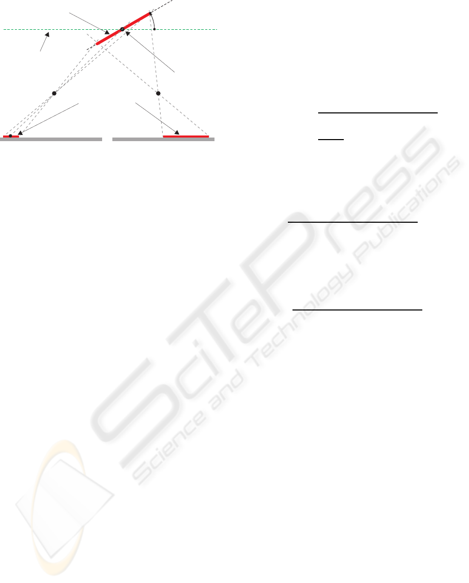
Figure 1: This image shows a schematic configuration of a
parallel stereo camera setting and a planar surface, 2-D top
view only.
following, we will sketch the derivations for planes,
spheres and cylinders. However, the method is ap-
plicable in an analogous way to other parametric sur-
faces.
2.2 Planar Model
In order to derive a formula for z
L
that depends on
planar model parameters, we describe a planar image
region (target plane) relative to a virtual plane paral-
lel to the CCD-chip. The planes differ by a rotation
at a certain anchor point about the x- and y-axis. Fig-
ure 1 shows a schematic top view. The anchor point
is specified in world coordinates and denoted with x
a
.
The orientation is specified via rotation angles about
the x-axis (α
x
) and y-axis (α
y
). Note that these two
rotations suffice to describe any possible plane orien-
tation. From analytical geometry, it can be derived
that points x
′
from the virtual plane are transformed
into points x on the rotated target plane by applying
the transformation matrix
T =
cosα
y
sinα
x
sinα
y
cosα
x
sinα
y
0 cosα
x
− sinα
x
− sinα
y
sinα
x
cosα
y
cosα
x
cosα
y
!
, (7)
leading to the following transformation formula
x = T

x
′
− x
a

+ x
a
. (8)
Because the virtual plane is parallel to the CCD-chip
of the camera, the z-coordinate for points on this fron-
toparallel plane is always equal to the z-coordinate of
the anchor point, z
′
= z
a
. Using this, we can rewrite
the transformation equation above to


x
y
z


= T


x
′
− x
a
y
′
− y
a
0


+


x
a
y
a
z
a


. (9)
With this, the depth z on the target plane, given the
anchor point and rotation angles, reads as
z = (y
′
− y
a
)sinα
x
cosα
y
− (x
′
− x
a
)sinα
y
+z
a
, (10)
where (x
′
− x
a
) and (y
′
− y
a
) can also be expressed
with their counterparts on the rotated target plane re-
arranging and substituting the transformation equa-
tions (9):
x
′
− x
a
=
x− x
a
− (y
′
− y
a
)sinα
x
sinα
y
cosα
y
(11)
y
′
− y
a
=
y− y
a
cosα
x
. (12)
Applying these two equations to the depth formula
(10) and replacing the 3-D world coordinates with
their 2-D chip projections (using the projection equa-
tions (4) and (5)) finally leads to
z
L
= f
x
a
sinα
y
− y
a
tanα
x
+ z
a
cosα
y
u
Lx
sinα
y
− u
Ly
tanα
x
+ f cosα
y
. (13)
With this we have an equation that describes z
L
in
terms of the parameters of a planar model. Substi-
tuting z
L
in the basic mapping equation (6) leads to
u
Rx
= u
Lx
−
b
u
Lx
sinα
y
− u
Ly
tanα
x
+ f cosα
y
x
a
sinα
y
− y
a
tanα
x
+ z
a
cosα
y
(14)
u
Ry
= u
Ly
. (15)
These equations allow for a mapping of the view of
a plane from the left camera to the right camera by
means of the planar parameters (z
a
, α
x
and α
y
). The
values for x
a
and y
a
can be chosen arbitrarily. They
just define at which position the depth z
a
of the pla-
nar model is estimated. Please note that the mapping
equations (14) and (15) for the planar model corre-
spond to the well-knownhomographytransformation.
This derivation was done in order to ease the under-
standing of the derivation of the other models, which
are the main focus of this paper.
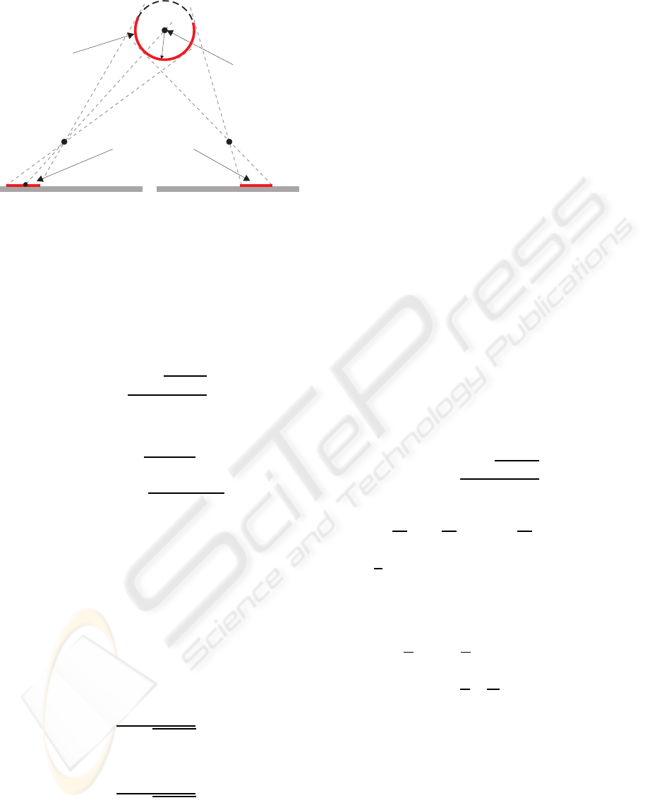
2.3 Spherical Model
In this section, we show that in our generic framework
it is possible to map other parametric surface models
starting with the sphere. As in section 2.2, we need
to formulate z
L
as a function of the parametric model.
A sphere in the three-dimensional space with radius r
can be described by
r
2
= (x− x
a
)
2
+ (y− y
a
)
2
+ (z− z
a
)
2
, (16)
where (x
a
, y
a
, z
a
) is the anchor point (center) of the
sphere. For a graphical explanation see figure 2. As
we have done with the planar equations in section 2.2,
DIRECT SURFACE FITTING
127

leftcamera
rightcamera
projections
anchor
(x
a
,y
a
,z
a
)
targetsphere
r
Figure 2: This image shows a schematic configuration of a
parallel stereo camera setting and a spherical surface, 2-D
top view only.
we replace the 3-D world points with their projections
on the CCD-chips using the projection equations (4)
and (5). As the replacement is straightforward we
omit it for brevity and proceed with the resulting for-
mula rearranged for z
L
z
L1,2
=
µ±
p
µ
2
− νλ
λ
, (17)
with
λ = 1+
u
2
Lx
+ u
2
Ly
f
2
(18)
µ = z
a
+
u
Lx
x
a
+ u
Ly
y
a
f
(19)
ν = x
2
a
+ y
2
a
+ z
2
a
− r
2
. (20)
At a first glance having two solutions in the spher-
ical depth equation (17) looks puzzling. In fact, a
closer look at figure 2 reveals that using the “−” in
the spherical depth equation (17) means mapping a
sphere (convex structure) and using the “+” means
mapping a bowl (concave structure). Therefore, sub-
stituting z
L
in the basic mapping equation (6) with the
spherical depth equation (17) leads to two transforma-
tion equations. The first is the equation for transform-
ing the view of a sphere
u
R
= u
L
−
bfλ
µ−
p
µ
2
− νλ

1
0

, (21)
and the second for transforming the view of a bowl
u
R
= u
L
−
bfλ
µ+
p
µ
2
− νλ

1
0

. (22)
These equations allow for a mapping of the view of
a sphere or a bowl from the left camera to the right
camera by means of the spherical model parameters
(z
a
, x
a
, y
a
and r).
2.4 Cylindrical Model
The derivation of the formulas for the cylindrical
model follows the same scheme like for the planar and
spherical model. Since the formulas get a bit lengthy,
the following derivation is just a brief sketch. The
setup of the cylindrical model is very similar to that
of the sphere (see figure 2). We have chosen to de-
scribe the cylindrical model by:
r
2
= (x− x
a
)
2
+ (z− z
a
)
2
, (23)
This means our cylindrical model is infinite in the
y-direction. In contrast to the spherical model, it
is necessary to incorporate a rotation matrix like we
have done for the planar model
T =
cosα
z
− sinα
z
0
cosα
x
sinα
z
cosα
x
cosα
z
− sinα
x
sinα
x
sinα
z
sinα
x
cosα
z
cosα
x
!
. (24)
For the cylindrical model, we have chosen the rota-
tion about the x-axis and the z-axis. This leads to six
parameters for the model of the cylinder with anchor
point (a
x
, a
y
, a
z
), rotation angles (α
x
, α
z
) and radius
r. Actually, the model has only five parameters as the
y-position for the infinitely expanded cylinder can be
fixed. For the derivation we proceed in a way anal-
ogous to the plane and the sphere (not shown in full
detail here). The resulting depth formula has a struc-
ture similar to that of the sphere
z
L1,2
=
τ±
p
τ
2
− ηκ
κ
, (25)
with
κ = u
2
Lx
A
f
2
+ u
2
Ly
B
f
2
+ 2u
Lx
u
Ly
C
f
2
+
2
f
(u
Ly
D+ u
Lx
E) + F
(26)
η = y
2
a
A+ x
2
a
B+ 2x
a
y
a
C+
2z
a
(y
a
D+ x
a
E) + z
2
a
F − r
2
(27)
τ = u
Ly
y
a
A
f
+ u
Lx
x
a
B
f
+
(u
Ly
x
a
+ u
Lx
y
a
)
C
f
+
z
a
f
(u
Ly
D+ u
Lx
E)+
y
a
D+ x
a
E + z
a
F ,
(28)
where
A = sinα
x
sinα
z
cosα
z
(29)
B = 1− cos
2
α
x
cos
2
α
z
(30)
C = cos
2
α
z
(31)
D = 1 − sin
2
α
x
cos
2
α
z
(32)
E = − sinα
x
cosα
x
cos
2
α
z
(33)
F = sinα
x
sinα
z
cosα
z
. (34)
VISAPP 2010 - International Conference on Computer Vision Theory and Applications
128

Substituting z
L
of the basic mapping equation (6) with
the cylindrical depth equation (25) leads to two trans-
formation equations
u
R
= u
L
−
bfκ
τ±
p
τ
2
− ηκ

1
0

. (35)
These equations allow for a mapping of the view of
a cylindrical shape from the left camera to the right
camera by means of the cylindrical model parameters
(x
a
, y
a
, z
a
, α
x
, α
z
and r). As was pointed out in sec-
tion 2.3, “−” corresponds to mapping concave struc-
tures and “+” corresponds to mapping convex struc-
tures.
3 MODEL PARAMETER
ESTIMATION
The basic idea of our approach is to incorporate mod-
els directly into the correspondence search, instead
of fitting models into depth or disparity data gained
from some local correspondence searches. For this
purpose, we derived the transformation equations of
the parametric models in the last section that describe
the perspective view changes of these models in a
stereo camera setting. We now search for the model
parameters of larger image regions that explain the
perspective view changes of these regions between
different camera images. For doing so we use the
Hooke-Jeeves (Hooke and Jeeves, 1961) optimization
method. Its objectiveis to minimize the error between
the original left view and the transformed right view.
Hooke-Jeeves is a direct search method (Lewis
et al., 2000) for optimizing (fitness) functions. Start-
ing from an initial parameter set, an iterative refine-
ment is conducted by sampling alternative parameter
sets around the current solution. From these alterna-
tive sets the best one is selected. If no better solution
is found, the step size is reduced. This is repeated un-
til a minimal step size has been reached. Here we use
the SAD between the original left image of a surface
and the transformed right image as the fitness func-
tion for the Hooke-Jeeves algorithm. This means that
the search algorithm tries to find those parameters of
a parametric surface that best predict the perspective
change between the left and right camera view. We
use SAD because it is less sensitive to outliers in the
image data compared to a quadratic measure.
It may seem unusual to use Hooke-Jeeves in-
stead of a classical optimization based on gradients.
However, direct search methods like Hooke-Jeeves
have several advantages over gradient based solu-
tions. First, gradient based approaches need a for-
mal description of the fitness gradient which is based
on the image gradients. These, however, can only
be approximated locally, e.g. by means of a Taylor
expansion (Habbecke and Kobbelt, 2005; Lucas and
Kanade, 1981). Because of this, gradient based ap-
proaches usually need to rely on a resolution pyramid.
There is no such necessity when using a direct search
method like Hooke-Jeeves, because it searches the pa-
rameter space by means of sampling. Second, it is
easy to replace one fitness function with another one,
i.e. it is straightforward to exchange the model (trans-
formation formulas) or objective function (matching
function). In contrast to this, the formulas in gradi-
ent based optimization regimes depend on the model
as well as on the used objective function. This means
that gradient formulas have to be re-derived when the
model or the objective function are changed. More-
over, the possible set of matching metrics is limited,
as for example a SAD is not derivable. Last but
not least, the Hooke-Jeeves optimization is numeri-
cally very stable for the method presented here, since
only simple arithmetic and trigonometric functions
are used for the transformations.
Notwithstanding its advantages, Hooke-Jeeves is
rarely used as it is considered inefficient. Compared
to gradient based approaches Hooke-Jeeves needs
more iterations. However, the overall speed depends
on the function to optimize. Especially, using gra-
dient based approaches on images is quite expensive
because for calculating the local gradients the im-
ages have to be filtered in each iteration. This fil-
tering is avoided when using a direct search method
like Hooke-Jeeves. In (Habbecke and Kobbelt, 2005)
a very efficient gradient method for plane estimation
was proposed which is about a factor of two to three
faster than the Levenberg-Marquardt minimization.
Their implementation needs roughly 15 iterations. On
an AMD Athlon 64 3500+ they need around 0.2ms
for one iteration of a patch of 1000 pixels, i.e. the
overall computation time is 3ms. In terms of itera-
tions our Hooke-Jeeves implementation is quite ex-
pensive as it usually needs on average 175 iterations.
However, on a comparable system (one core of an In-
tel Xeon X5355) the overall computation time for a
patch of 1000 pixels is 6.8ms. This demonstrates that
Hooke-Jeeves can compete with state-of-the-art gra-
dient based optimization when it comes to plane fit-
ting.
4 RESULTS
In order to prove the concept of our approach and
to evaluate the accuracy of the parameter estimation,
we conducted some experiments with virtual scenes.
DIRECT SURFACE FITTING
129

Ground Truth Estimated
α
x
+37
◦
+37.00
◦
α
y
−23
◦
−22.81
◦
z
a
500mm 499.70mm
(a) Plane
Ground Truth Estimated
x
a
150mm 149.32mm
y
a
−70mm −69.14mm
z
a
500mm 500.32mm
r 100mm 100.08mm
(b) Sphere
Ground Truth Estimated
x
a
−150mm −150.76mm
y
a
0mm 0.00mm
z
a
500mm 500.21mm
α
x
−31
◦
−31.62
◦
α
z
−13
◦
−11.18
◦
r 70mm 69.61mm
(c) Cylinder
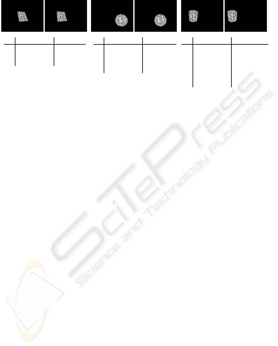
Figure 3: Results of our approach applied on the three different rendered objects a) Plane b) Sphere and c) Cylinder. The
images at the top show the left and right camera image of the different objects. The tables below the images show the ground
truth parameters of the objects and the parameters estimated with our approach.
To this end, we rendered camera images by means of
POVRay (http://www.povray.org/), a free ray-tracing
program. We rendered the images such that they cor-
responded to a standard parallel stereo camera setting.
The objects were places in a distance of 50cm in front
of the stereo cameras. Figure 3 depicts the rendered
images and the results achieved by our approach.
Comparing the ground truth values of the param-
eters with the estimated parameter values shows that
our approach is able to estimate the model parame-
ters very precisely. Although the objects cover only
image regions of about 100 × 100 pixels, angles are
estimated up to a half degree for the plane and up to
two degrees for the cylinder and positions and radii
up to one mm.
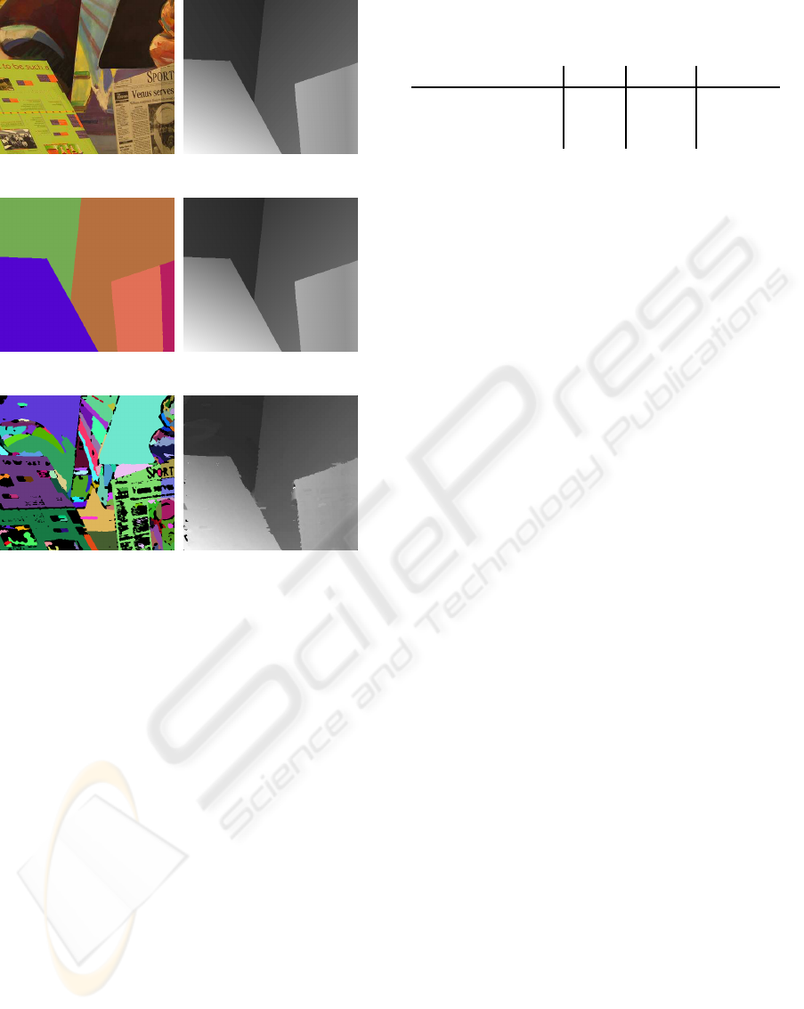
In order to evaluate the precision of our approach
under more realistic conditions, we used the Venus
scene from the Middlebury data set (Scharstein and
Szeliski, 2003). This scene consists of five planar sur-
faces. We segment the left image into the five planar
regions (figure 4c) in order to estimate planar param-
eters for each. Note that we segment only the left
image, as the search process warps the right image
into the left image for comparison. Afterwards we
compute a disparity map from the estimated param-
eters. The results are shown in figure 4. Comparing
the ground truth (figure 4b) and the estimated dispar-
ity map (figure 4d) reveals almost no errors. The per-
centage of bad pixels, with an accuracy of 0.5 pixels,
is 0.00%, i.e. no erroneous estimations. The percent-
age of bad pixels is the common error measure used
to compare results on the Middlebury data set and is
described in (Scharstein and Szeliski, 2003). How-
ever, we segmented the image by hand. A standard
segmentation algorithm may produce a lot more seg-
ments of poorer quality. It is a common assumption
in the field of computer vision that homogeneous re-
gions are likely to be planes. Hence, we used a sim-
ple region growing algorithm in order to segment the
Venus scene. Figure 4e shows that such a segmen-
tation leads to a large number of regions of differ-
ent sizes. Note that regions smaller than 100 pix-
els are displayed in black. Although this automated
preprocessing constitutes quite a challenge for our
algorithm, it is still able to produce a good estima-
tion. The percentage of bad pixels (accuracy 0.5 pix-
els) is 1.39%. This shows that our algorithm is able
to estimate model parameters for imperfect and even
very small segments as long as the model assumption
holds.
For the other models it is much harder to provide
a reasonable segmentation. Hence, we investigated if
a model selection is possible for a given segment. For
this purpose, we had a closer look on what we call
the residual error. The residual error is the difference
between the original left image and the transformed
right image, using the parameters estimated by our al-
gorithm. This means that the residual error is the min-
imal value of the fitness function that has been found
by Hooke-Jeeves. However, using the same model
the residual error varies substantially for different sur-
faces. The problem arises mainly from the fact that
we use SAD for image comparison. Hence, the resid-
ual error tends to be larger for surfaces of high con-
trast. It has to be analyzed in future work if other ob-
jective functionsare more suitable. For example using
a normalized cross-correlation would make the resid-
ual error more descriptive. Because of the variation of
the residual error over different surfaces, we decided
to compare the residual error of different models. Ta-
ble 1 shows the residual error of the planar, spherical
and cylindrical model applied to the three POVRay
VISAPP 2010 - International Conference on Computer Vision Theory and Applications
130

(a) (b)
(c) (d)
(e) (f)
Figure 4: Results on the Venus scene from the Middlebury
data set. a) Left camera image, b) ground truth disparity,
c) segmentation of the image by hand and e) image seg-
mentation into homogeneous regions using region grow-
ing. d) and f) show the disparity maps produced by our
approach. Here we applied the planar model to each seg-
mented region and calculated disparity values from the es-
timated parameters.
rendered objects plane, sphere and cylinder shown in
figure 3. The results show a clear difference between
the residual error of the correct and wrong models. In
most cases the residual error of the wrong models is a
magnitude larger than the residual error of the correct
model. This means that the correct model can be cho-
sen by taking the one with the smallest residual error.
The only exception is the relatively low residual er-
ror of the cylindrical model on the plane object. The
reason is that the cylindrical model is able to approx-
imate a planar surface well by using a large radius.
Although the same argument applies to the spherical
model the maximal step sizes used for Hooke-Jeeves
restricted such an approximation.
In the last two experiments, we used a real stereo
camera system in order to acquire stereo images of
real-world objects under real-world conditions. Un-
fortunately, only partial ground truth data is available
Table 1: Comparison of the residual errors (SAD per pixel)
of the three different models applied to the three different
objects.
Plane Sphere Cylinder
Planar Model 3.38 29.73 24.34
Spherical Model 14.45 5.19 22.02
Cylindrical Model 7.90 23.44 6.08
here. Figure 5 shows the stereo images of a box, a ball
and a can. Below the images of the ball and the can
the estimated radius is compared to the radius mea-
sured by hand. As you can see the estimation is quite
accurate despite of the fact that the objects are really
small in size. Comparing the rotation angle α
x
of the
front face with that of the top face of the box shows
that the faces differ approximately by 85
◦
. This is
very close to the 90
◦
the faces should differ and is a
strong indicator that the estimation was correct. In or-
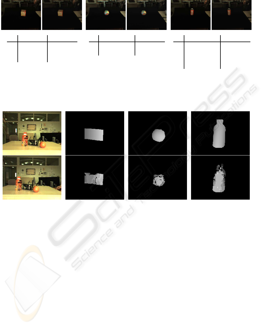
der to get an impression of how our approach works
with imperfect objects and cluttered scenes, we ar-
ranged a scene with an apple, a bottle and a box. Fig-
ure 6 shows that scene and the estimated disparities
of our approach compared to disparities extracted us-
ing a standard block matching stereo approach with
normalized cross-correlation. For better visibility, we
zoomed in the disparity map and removed the back-
ground using the object masks. The results show that
our approach is able to produce very smooth disparity
maps compared to the standard approach. Although
the apple and the bottle do not have the exact shape
of a sphere and a cylinder our approach is able to
fit the models and produce reasonable depth results.
Furthermore, matching large regions enhances robust-
ness against clutter in the background and reduces the
aperture problem.
5 SUMMARY
In this paper, we presented a method which is able
to fit 3-D surface models directly in stereo camera
images. This is in contrast to the usual approach
of fitting models in the disparity data, calculated in
advance with a standard stereo method. Prior ap-
proaches that fit 3-D surfaces directly to the im-
ages are usually restricted with respect to the sur-
face model, camera model or objective function. The
major difference in our approach is that we use the
Hooke-Jeeves optimization instead of a classical op-
timization method based on derivatives. This enables
literally arbitrary surface models, camera models and
objective functions. We demonstrated this by deriv-
ing formulas for a planar, a spherical and a cylindri-
cal model. Using rendered scenes, we showed that
DIRECT SURFACE FITTING
131

Top Face Front Face
α
x
+48.48
◦
−36.92
◦
α
y
+8.44
◦
+15.11
◦
z
a
496.52mm 498.76mm
(a) Box
Ground Truth Estimated
r 49.30mm 53.98mm
z
a
∼ 525mm 542.19mm
(b) Ball
Ground Truth Estimated
r 35.00mm 35.40mm
z
a
∼ 540mm 542.84mm
α
x
—– −23.64
◦
α
z
—– +0.30
◦
(c) Can
Figure 5: Results of our approach applied to three different real world objects a) Box b) Ball and c) Can. The images at the
top show the left and right camera image of the different objects. The tables below the Ball and the Can show the ground truth
radius compared to the estimated radius. For the Box the result for the two visible faces are shown, the estimations show that
the angle between them is close to 90
◦
.
(a) Office scene (b) Box disparity (c) Apple disparity (d) Bottle disparity
Figure 6: This figure shows the results of our approach compared to a standard stereo approach. a) Top and bottom image
show the left and right stereo image, respectively. b-d) Close-ups of the disparities for the three objects Box, Apple and Bottle.
The top row shows the disparity maps of our approach and the bottom row the results of a standard block matching stereo
approach with normalized cross-correlation.
model parameters are estimated very accurately. Fur-
thermore, we showed that our approach works well
under real-world conditions.
In future work, we want to derive formulas for
mapping further models, like cones and ellipsoids.
With such a set of models available a wide range of
applications is conceivable. For example the fitting
can be used to generate a coarse pre-classification to
aid object recognition. Another important point for
future work is to conduct a more elaborated analysis
of the accuracy of the parameter estimation and the
impact of occlusion. Last but not least, we want to
analyze the influence of different objective functions
on the robustness and accuracy of the parameter esti-
mation.
REFERENCES
Baker, S., Szeliski, R., and Anandan, P. (1998). A layered
approach to stereo reconstruction. In Proceedings of
the IEEE Computer Society Conference on Computer
Vision and Pattern Recognition, pages 434–441.
Bleyer, M. and Gelautz, M. (2005). Graph-based surface
reconstruction from stereo pairs using image segmen-
tation. In Videometrics VIII, volume 5665, pages 288–
299.
Cernuschi-Frias, B., Cooper, D. B., Hung, Y.-P., and Bel-
humeur, P. N. (1989). Toward a model-based bayesian
theory for estimating and recognizing parameterized
3-d objects using two or more images taken from dif-
ferent positions. IEEE Transactions on Pattern Anal-
ysis and Machine Intelligence, 11(10):1028–1052.
Habbecke, M. and Kobbelt, L. (2005). Iterative multi-
view plane fitting. In Vision, Modeling, Visualization
VMV’06, pages 73–80.
VISAPP 2010 - International Conference on Computer Vision Theory and Applications
132

Habbecke, M. and Kobbelt, L. (2007). A surface-growing
approach to multi-view stereo reconstruction. Com-
puter Vision and Pattern Recognition, pages 1–8.
Hartley, R. and Zisserman, A. (2004). Multiple View Geom-
etry in Computer Vision. Cambridge University Press,
second edition.
Hirschm¨uller, H. (2006). Stereo vision in structured envi-
ronments by consistent semi-global matching. In Pro-
ceedings of the IEEE Computer Society Conference on
Computer Vision and Pattern Recognition, volume 2,
pages 2386–2393.
Hooke, R. and Jeeves, T. A. (1961). ”Direct Search” Solu-
tion of Numerical and Statistical Problems. Journal of
the Association for Computing Machinery, 8(2):212–
229.
Klaus, A. S., Sormann, M., and Karner, K. (2006).
Segment-based stereo matching using belief propaga-
tion and a self-adapting dissimilarity measure. In Pro-
ceedings of the 18th International Conference on Pat-
tern Recognition, pages 15–18.
Lewis, R. M., Torczon, V., and Trosset, M. W. (2000). Di-
rect search methods: Then and now. Journal of Com-
putational and Applied Mathematics, 124:191–207.
Lucas, B. D. and Kanade, T. (1981). An iterative image
registration technique with an application to stereo vi-
sion. In International Joint Conference on Artificial
Intelligence, pages 674–679.
Okutomi, M., Nakano, K., Maruyama, J., and Hara, T.
(2002). Robust estimation of planar regions for visual
navigation using sequential stereo images. In Pro-
ceedings of the 2002 IEEE International Conference
on Robotics and Automation, pages 3321–3327.
Scharstein, D. and Szeliski, R. (2003). High-accuracy
stereo depth maps using structured light. In Proceed-
ings of the IEEE Computer Society Conference on
Computer Vision and Pattern Recognition, volume 1,
pages 195–202, Madison, WI,.
Wang, Z. F. and Zheng, Z. G. (2008). A region based stereo
matching algorithm using cooperative optimization.
In Proceedings of the IEEE Computer Society Con-
ference on Computer Vision and Pattern Recognition,
pages 1–8.
DIRECT SURFACE FITTING
133