
TRACKING OF FACIAL FEATURE POINTS BY COMBINING
SINGULAR TRACKING RESULTS WITH
A 3D ACTIVE SHAPE MODEL
Moritz Kaiser, Dejan Arsi
´
c, Shamik Sural and Gerhard Rigoll
Technische Universit
¨
at M
¨
unchen, Arcisstr. 21, 80333 Munich, Germany
Keywords:
Facial feature tracking, 3D Active Shape Model, Face pose estimation.
Abstract:
Accurate 3D tracking of facial feature points from one monocular video sequence is appealing for many
applications in human-machine interaction. In this work facial feature points are tracked with a Kanade-Lucas-
Tomasi (KLT) feature tracker and the tracking results are linked with a 3D Active Shape Model (ASM). Thus,
the efficient Gauss-Newton method is not solving for the shift of each facial feature point separately but for the
3D position, rotation and the 3D ASM parameters which are the same for all feature points. Thereby, not only
the facial feature points are tracked more robustly but also the 3D position and the 3D ASM parameters can be
extracted. The Jacobian matrix for the Gauss-Newton optimization is split via chain rule and the computations
per frame are further reduced. The algorithm is evaluated on the basis of three handlabeled video sequences
and it outperforms the KLT feature tracker. The results are also comparable to two other tracking algorithms
presented recently, whereas the method proposed in this work is computationally less intensive.
1 INTRODUCTION
Accurate 3D tracking of facial feature points from
one monocular video sequence is a challenging task,
since only 2D information is available from the video.
The 3D tracking is appealing for many applications in
human-machine interaction. In contrast to 2D track-
ing, information about the 3D head position and the
3D head movement can be extracted and it is also pos-
sible to perform pose independent emotion and ex-
pression recognition (Gong et al., 2009). Statistical
models are a powerful tool for solving this task. Of-
ten, models that are based on the entire appearance
of faces are employed (Cootes et al., 1998; Faggian
et al., 2008). Nevertheless, for many applications it
is sufficient to track only a certain number of selected
facial feature points. The advantage of only tracking
a sparse set of points is that it is less complicated and
computationally less intensive.
1.1 Conception of this Work
For model-free 2D tracking the Kanade-Lucas-
Tomasi (KLT) (Tomasi and Kanade, 1991) feature
tracker generates reasonable results and it is compu-
tationally efficient. The KLT feature tracker is a lo-
cal approach that computes the shift of each facial
feature point separately. Often due to noise, illu-
mination changes or weakly textured neighborhood
the KLT feature tracker loses track of some feature
points. An unrealistic constellation of points is the
result as depicted in Figure 1. In this work we com-
bine the tracking results for each single point with a
3D Active Shape Model (ASM). The 3D ASM guar-
antees a certain structure between the locally tracked
points. Hence, the efficient Gauss-Newton optimiza-
tion (Bertsekas, 1999) is not solving for the 2D shift
of several facial feature points separately but for the
parameters of a 3D ASM and rotation, translation and
scale parameters which are the same for all feature
points. Thereby, not only the facial feature points are
tracked more robustly but also additional information
like the parameters of the 3D ASM for emotion and
expression recognition and the 3D head position and
movement are extracted.
1.2 Previous Work
Model-free tracking algorithms are not suitable for
extracting 3D information from a monocular video
sequence. Thus, model-based methods are applied.
A popular approach for tracking is to use statistical
281
Kaiser M., Arsi
´
c D., Sural S. and Rigoll G. (2010).
TRACKING OF FACIAL FEATURE POINTS BY COMBINING SINGULAR TRACKING RESULTS WITH A 3D ACTIVE SHAPE MODEL.
In Proceedings of the International Conference on Computer Vision Theory and Applications, pages 281-286
DOI: 10.5220/0002819302810286
Copyright
c
SciTePress

models based on the entire appearance of the face.
The method described in (Cristinacce and Cootes,
2006a) uses texture templates to locate and track fa-
cial features. In (Cristinacce and Cootes, 2006b) tex-
ture templates are used to build up a constrained lo-
cal appearance model. The authors of (Sung et al.,
2008) propose a face tracker that combines an Active
Appearance Model (AAM) with a cylindrical head
model to be able to cope with cylindrical rotation. In
(Fang et al., 2008) an optical flow method is com-
bined with a statistical model, as in our approach.
However, the optical flow algorithm by (Brox et al.,
2004) is applied which is computationally more inten-
sive than a Gauss-Newton optimization for only sev-
eral facial feature points. All those methods rely on
statistical models that are based on the entire texture
of the face which is computationally more intensive
than statistical models based on only a sparse set of
facial feature points.
The authors of (Heimann et al., 2005) employed
a statistical model which is based only on a few fea-
ture points, namely a 3D Active Shape Model, which
is directly matched to 3D point clouds of organs for
detection. The matching takes from several minutes
up to several hours. (Tong et al., 2007) use a set of fa-
cial feature points whose spatial relations are modeled
with a 2D hierarchical shape model. Multi-state local
shape models are used to model small movements in
the face.
This paper is organized as follows. In Section
2 our algorithm is presented, where first a track-
ing framework for a generic parametric model is ex-
plained and then the 3D parametric model we employ
is described. Quantitative and qualitative results are
given in Section 3. Section 4 gives a conclusion and
outlines future work.
2 PROPOSED ALGORITHM
In this section, a tracking framework is illustrated,
that can be applied if the motion can be described by
a parametric model. The least-squares estimation of
the parameters of a generic parametric model is ex-
plained. Subsequently, the parametric model that is
employed in this work, namely a 3D ASM, is pre-
sented. It is explained how the parameter estimation,
that has to be performed for each frame, can be carried
out more efficiently. Furthermore, some constraints
on the parameter estimation are added.
Following the ISO typesetting standards, matri-
ces and vectors are denoted by bold letters (I, x) and
scalars by normal letters (I, t).
2.1 Tracking Framework for
Parametric Models
Assume that the first frame of a video sequence is ac-
quired at time t
0
= 0. Vector x
i
= (x, y)
T
describes the
location of point i in a frame. The location changes
over time according to a parametric model x
i
(µ
t
),
where µ
t
is the parameter vector at time t. The set
of points for which the parameter vector is supposed
to be the same is denoted by T = {x
1
,x
2
,...,x
N
}. It
is assumed that the position of the N points and thus
also the parameters µ
0
for the first frame are known.
The brightness value of point x
i
(µ
0
) in the first frame
is denoted by I(x
i
(µ
0
),t
0
= 0).
The brightness constancy assumption implies that
at a later time the brightness of the point to track is
the same
I(x
i
(µ
0
),0) = I(x
i
(µ
t
),t). (1)
For better readability we write I
i
(µ
0
,0) = I
i
(µ
t
,t). The
energy function that has to be minimized at every time
step t for each location i in order to obtain µ
t
is
E
i
(µ
t
) =
I
i
(µ
t
,t)− I
i
(µ
0
,0)
2
. (2)
Knowing µ
t
at time t, we only need to compute ∆µ in
order to determine µ
t+τ
= µ
t
+ ∆µ. The energy func-
tion becomes
E
i
(∆µ) =
I
i
(µ
t
+ ∆µ,t + τ) − I
i
(µ
0
,0)
2
. (3)
If τ is sufficiently small, I
i
(µ
t
+ ∆µ,t + τ) can be lin-
earized with a Taylor series expansion considering
only the first order term and ignoring the second and
higher order terms
I
i
(µ
t
+ ∆µ,t + τ)
≈ I
i
(µ
t
,t)+
∂
∂µ
I
i
(µ
t
,t)· ∆µ + τ
∂
∂t
I
i
(µ
t
,t), (4)
with
∂
∂µ
I =
∂
∂µ
1
I,
∂
∂µ
2
I, . . . ,
∂
∂µ
N
p
I
. By approximating
τ
∂
∂t
I
i
(µ
t
,t) ≈ I
i
(µ
t
,t + τ) − I
i
(µ
t
,t), (5)
Equation (3) becomes
E
i
(∆µ)
=
∂
∂µ
I
i
(µ
t
,t)· ∆µ + I
i
(µ
t
,t + τ) − I
i
(µ
0
,0)
2
. (6)
The error is defined as
e
i
(t + τ) = I
i
(µ
t
,t + τ) − I
i
(µ
0
,0). (7)
If we assume that E
i
is convex, the minimization prob-
lem can be solved by
∂
∂∆µ
E
i
=
∂
∂µ
I
i
(µ
t
,t)· ∆µ + e
i
(t + τ)
·
∂
∂µ
I
i
(µ
t
,t) = 0. (8)
VISAPP 2010 - International Conference on Computer Vision Theory and Applications
282

Figure 1: The facial feature points of the left image are
tracked by a KLT feature tracker. In the right image it can
be seen that one facial feature point (white cross) drifted off.
Taking into account all points i, the system of linear
equations can be solved for ∆µ by
∆µ = −(J
T
J)
−1
J
T
e(t + τ), (9)
where
e(t + τ) =
e
1
(t + τ)
.
.
.
e
N
(t + τ)
. (10)
J denotes the N × N
p
Jacobian matrix of the image
with respect to µ:
J =
∂
∂µ
I
1
(µ
t
,t)
.
.
.
∂
∂µ
I
N
(µ
t
,t)
, (11)
where N is the number of points with equal parame-
ters and N
p
is the number of parameters.
For the KLT feature tracker there are only two
parameters to estimate, namely the shift in x- and
y-direction.
∂
∂x
I
i
(µ
t
,t) can be estimated numerically
very efficiently with e.g. a Sobel filter. The set T
for which equal parameters are assumed is a squared
neighborhood around the feature point that should
be tracked. For the case of tracking several facial
feature points, each facial feature point would have
to be tracked separately. Although the KLT feature
tracker works already quite well, single points to track
might drift off due to a weakly textured neighborhood,
noise, illumination changes or occlusion. Figure 1
(left) shows the first frame of a video sequence with
22 feature points and Figure 1 (right) illustrates the
tracked points several frames later. Most of the fea-
ture points are tracked correctly but one (marked with
a white cross) got lost by the feature tracker. The
human viewer can immediately see that the spacial
arrangement of the facial feature points (white and
black crosses) is not typical for a face. The structure
between the facial feature points can be ensured by a
parametric model. In the case of landmarks on a face
a 3D ASM seems appropriate.
Figure 2: Multiple views of one 3D facial surface. The fa-
cial feature points are manually labeled to build up a 3D
ASM.
2.2 3D Active Shape Model
The 2D ASM was presented in (Cootes et al., 1995).
The 3D ASM can be described analogously. An ob-
ject is specified by N feature points. The feature
points are manually labeled in N
I
training faces, as
shown in Figure 2 exemplary for one 3D facial sur-
faces. The 3D point distribution model is constructed
as follows. The coordinates of the feature points are
stacked into a shape vector
s =
x
1
,y
1
,z
1
,...,x
N
,y
N
,z
N
. (12)
The 3D shapes of all training images can be aligned
by translating, rotating and scaling them with a Pro-
crustes analysis (Cootes et al., 1995) so that the sum
of squared distances between the positions of the fea-
ture points is minimized. The mean-free shape vec-
tors are written column-wise into a matrix and princi-
pal component analysis is applied on that matrix. The
eigenvectors corresponding to the N
e
largest eigenval-
ues λ
j
are concatenated in a matrix U =
u
1
|...|u
N
e
.
Thus, a shape can be approximated by only N
e
param-
eters:
s ≈ M(α) = ¯s +U · α, (13)
where α is a vector of N
e
model parameters and ¯s is
the mean shape. We denote the 3D ASM by the 3N-
dimensional vector
M(α) =
M
1
(α)
.
.
.
M
N
(α)
; M
i
(α) =
M
x,i
(α)
M
y,i
(α)
M
z,i
(α)
. (14)
The parameters α describe the identity of an in-
dividual and its current facial expression. Addition-
ally, we assume that the face is translated in x- and
y-direction by t
x
and t
y
, rotated about the y- and z-axis
by θ
y
and θ
z
, and scaled by s. The scaling is a sim-
plified way of simulating a translation in z-direction,
where it is assumed that the z-axis comes out of the
2D image plane. Thus, the model we will employ be-
comes
x
i
(µ) = sR(θ
y
,θ
z
)M
i
(α) +
t
x
t
y
, (15)
TRACKING OF FACIAL FEATURE POINTS BY COMBINING SINGULAR TRACKING RESULTS WITH A 3D
ACTIVE SHAPE MODEL
283

where µ = (s,θ
y
,θ
z
,t
x
,t
y
,α) is the (5 + N
e
)-
dimensional parameter vector and
R(θ
y
,θ
z
)
=
cosθ
y
cosθ
z
cosθ
y
sinθ
z
−sinθ
y
−sinθ
y
cosθ
z
0
. (16)
We directly insert the 3D ASM of Equation 15 into
our tracking framework for parametric models of
Equation 9 in order to estimate the parameters µ
t
in
a least-squares sense for each frame.
2.3 Efficient Parameter Estimation
Since J of Equation 9 depends on time-dependent
quantities, it must be recomputed for each frame. Es-
pecially for the model of Equation 15 the numerical
computation of
∂
∂µ
I(µ
t
,t) at each time step is time con-
suming. Therefore, the derivative of the image with
respect to the parameters is decomposed via chain
rule into an easily computable spatial derivative of the
image and a derivative of the parametric model with
respect to the parameters which can be solved analyt-
ically. Additionally, if, as in Equation 1, it is assumed
that
∂
∂x
I
i
(µ
t
,t) =
∂
∂x
I
i
(µ
0
,0), we obtain
J =
∂
∂x
I
1
(µ
0
,0)
∂
∂µ
x
1
(µ
t
)
.
.
.
∂
∂x
I
N
(µ
0
,0)
∂
∂µ
x
N
(µ
t
)
. (17)
The numerical derivative
∂
∂x
I
i
(µ
0
,0) and the analyti-
cal derivative
∂
∂µ
x
i
(µ
t
) can be computed offline. Thus,
for each frame the current estimation of µ has to be
plugged in the Jacobian matrix and the new parame-
ters are computed according to Equation 9.
2.4 Constraints on the 3D ASM
In order to prevent unrealistic results several con-
straints on the parameters are added. We require the
rotation θ
y
,θ
z
and also the 3D ASM parameters α not
to become too large:
θ
y
σ
2
θ
y
= −
∆θ
y
σ
2
θ
y
;
θ
z
σ
2
θ
z
= −
∆θ
z
σ
2
θ
z
(18)
α
j
σ
2
α
j
= −
∆α
j
σ
2
α
j
. (19)
We also require all parameters not to change too much
from one frame to another
∆µ
j
σ
2
∆µ
j
= 0. (20)
The constraints can easily be appended at the bottom
of J as further equations that the parameters ∆µ have
to satisfy. In order to have the right balance between
all equations, the equations of (9) are multiplied by
1/σ
2
N
, where σ
2
N
is the variance of the error e
i
. Note
that σ
2
α
j
can be directly taken from the principal com-
ponent analysis performed for the 3D ASM, while the
other variances have to be estimated.
2.5 Coarse-To-Fine Refinement
The coarse-to-fine refinement is a widely-used strat-
egy to deal with larger displacements for optical flow
and correspondence estimation. In practice, E
i
is of-
ten not convex as we have assumed in Equation 8. Es-
pecially, if there is a large displacement of the facial
feature points between two consecutive frames, the
least-squares minimization converges to only a local
minimum instead of the global minimum. This prob-
lem can be - at least partially - overcome by applying
a Gaussian image pyramid that has to be created for
each new frame. The computation of the parameter
vector is performed for the coarsest level. Then, the
parameters are taken as starting values for the next
finer level for which the computation is performed
again, and so on.
3 EXPERIMENTAL RESULTS
We built the 3D ASM from the Bosphorus Database
(Savran et al., 2008) where we used 2761 3D images
from 105 individuals. The images are labeled with
N = 22 facial feature points (Figure 2). Four pyramid
levels were employed for the Gaussian image pyra-
mid. On a 3GHz Intel
R
Pentium
R
Duo-Core proces-
sor and 3GB working memory the computation of the
parameters took on average 9.83 ms per frame.
3.1 Quantitative Evaluation
The proposed algorithm was evaluated on the basis
of three video sequences, each lasting roughly one
minute. In each video sequence an individual per-
forms motions, such as translation, rotation about the
y- and z-axis and it also changes the facial expres-
sion. The image resolution of the video sequence is
640 × 480 pixels. Every 10th frame was manually an-
notated with 22 landmarks and those landmarks were
used as ground truth. For each labeled frame the pixel
displacement d
i
=
p
∆x
2
+ ∆y
2
between the location
estimated by our algorithm and the ground truth was
computed. The pixel displacement was averaged over
VISAPP 2010 - International Conference on Computer Vision Theory and Applications
284
video sequence no. 1
0 100 200 300 400 500 600 700
0
10
20
frame
pixel displacement
our algorithm
KLT tracker
video sequence no. 2
0 50 100 150 200 250 300 350
5
10
15
frame
pixel displacement
our algorithm
KLT tracker
video sequence no. 3
0 50 100 150 200 250 300 350 400
0
20
40
frame
pixel displacement
our algorithm
KLT tracker
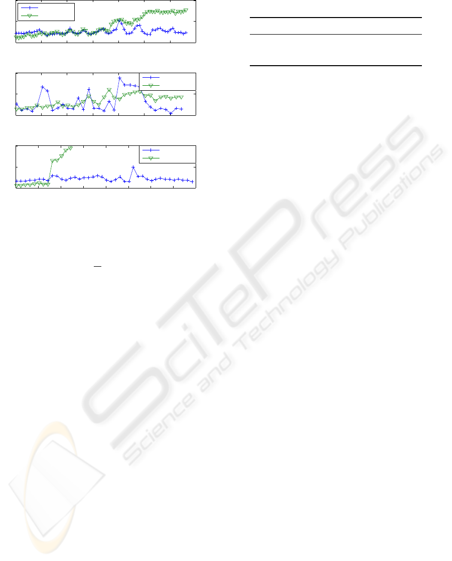
Figure 3: Pixel displacement for three test video sequences.
the N = 22 facial feature points:
D =
1
N
N
∑
i=1
d
i
. (21)
Figure 3 shows the results for the three video se-
quences. As a baseline system the KLT feature tracker
was chosen. Observe that already for the first frame
there is a small pixel displacement indicating that a
portion of the displacement is owed to the fact that
the annotation cannot always be performed unequiv-
ocally. For higher frame numbers the KLT feature
tracker loses track of some points and thus the pixel
displacement accumulates. Our algorithm is able
to prevent this effect and shows robust performance
over the whole sequence. In Table 1, the pixel dis-
placement averaged over all labeled frames of a se-
quence is depicted. Our algorithm outperforms the
KLT tracker. The results are also comparable with the
results reported recently by other authors. (Tong et al.,
2007) tested their multi-stage hierarchical models on
a dataset of 10 sequences with 100 frames per se-
quence. Considering that their test sequences had half
of our image resolution their pixel displacement is
similar to ours. Also the pixel displacement that (Fang
et al., 2008) reported for their testing database of 2
challenging video sequences is comparable to ours.
However, both methods are computationally consid-
erably more intensive than our tracking scheme.
3.2 Qualitative Evaluation
Figure 4 shows two sample frames of video sequence
no. 1. (The 3 video sequences are available together
Table 1: Pixel displacement averaged over a whole video
sequence.
video sequence no. 1 no. 2 no. 3
KLT tracker 8.07 8.45 43.34
our algorithm 5.19 8.03 8.71
in a single file as supplementary material.) The in-
formation box on the lower left corner shows posi-
tion details. For the left image it can be observed that
the rotation about the z-axis is detected correctly and
in the right image the rotation about the y-axis is es-
timated properly. Generally, it can be qualitatively
confirmed that not only the points are tracked reli-
ably in the 2D video sequence but also 3D motion
and expressions can be extracted from the sequence.
It is also important to notice that our 3D ASM works
with a relatively small number of facial feature points,
since the 3D faces of the Bosphorus Database are la-
beled with only 22 landmarks. In contrast, current 2D
face databases have more landmarks, some of them
roughly hundred points. It is expected that a 3D ASM
with more points would further improve the tracking
and parameter estimation results.
4 CONCLUSIONS AND FUTURE
WORK
A method for 3D tracking of facial feature points from
a monocular video sequence is presented. The fa-
cial feature points are tracked with a simple Gauss-
Newton estimation scheme and the results are linked
with a 3D ASM. Thus, the efficient Gauss-Newton
minimization computes the 3D position, rotation and
3D ASM parameters instead of the shift of each fea-
ture point separately. It is demonstrated how the
amount of computations that must be performed for
each frame can be further reduced. Results show that
the algorithm tracks the points reliably for rotation,
translations, and facial expressions. It outperforms
the KLT feature tracker and delivers results compa-
rable to two other methods published recently, while
being computationally less intensive.
In our ongoing research we will analyze the effect
of using gradient images and Gabor filtered images
to further improve the tracking results. We have also
planned to integrate a weighting matrix that depends
on the rotation parameters to reduce the influence of
facial feature points that might disappear.
TRACKING OF FACIAL FEATURE POINTS BY COMBINING SINGULAR TRACKING RESULTS WITH A 3D
ACTIVE SHAPE MODEL
285
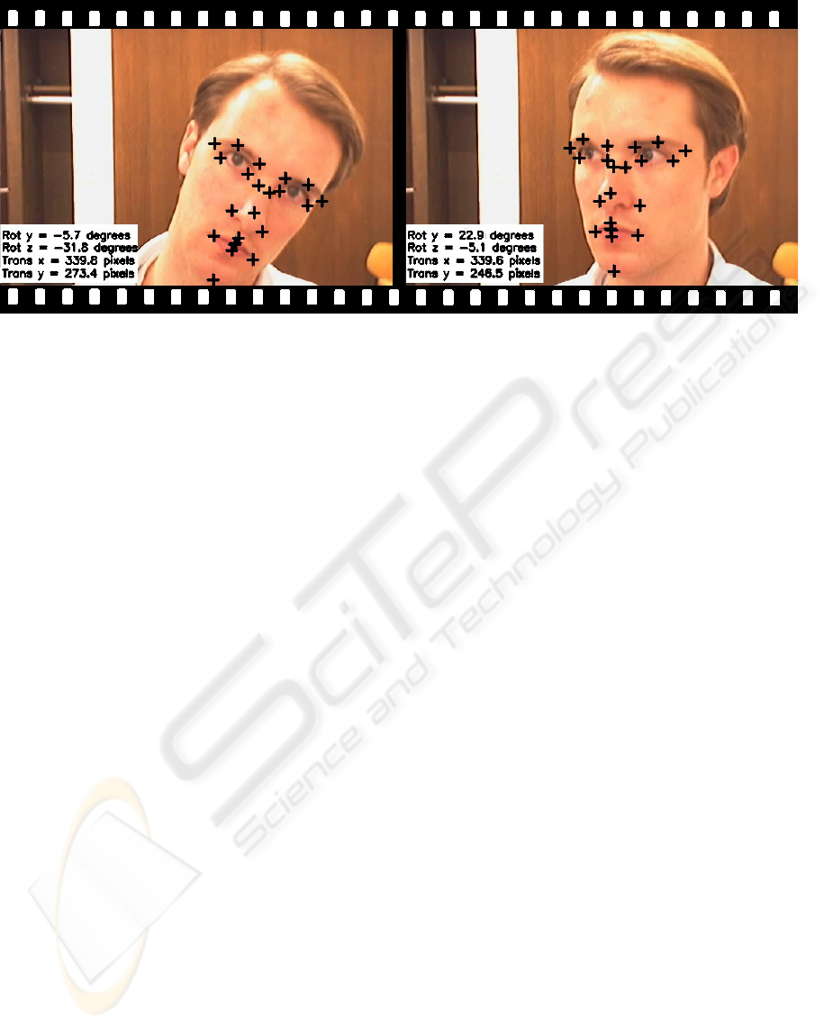
Figure 4: Features tracked by our algorithm. The information box shows rotation and translation parameters.
REFERENCES
Bertsekas, D. P. (1999). Nonlinear Programming. Athena
Scientific, 2nd edition.
Brox, T., Bruhn, A., Papenberg, N., and Weickert, J. (2004).
High accuracy optical flow estimation based on a the-
ory for warping. In ECCV (4), pages 25–36.
Cootes, T. F., Edwards, G. J., and Taylor, C. J. (1998). Ac-
tive appearance models. In ECCV (2), pages 484–498.
Cootes, T. F., Taylor, C. J., Cooper, D. H., and Graham,
J. (1995). Active shape models — their training and
application. CVIU, 61(1):38–59.
Cristinacce, D. and Cootes, T. F. (2006a). Facial feature
detection and tracking with automatic template selec-
tion. In FG, pages 429–434.
Cristinacce, D. and Cootes, T. F. (2006b). Feature detection
and tracking with constrained local models. In BMVC,
pages 929–938.
Faggian, N., Paplinski, A. P., and Sherrah, J. (2008). 3d
morphable model fitting from multiple views. In FG,
pages 1–6.
Fang, H., Costen, N., Cristinacce, D., and Darby, J. (2008).
3d facial geometry recovery via group-wise optical
flow. In FG, pages 1–6.
Gong, B., Wang, Y., Liu, J., and Tang, X. (2009). Auto-
matic facial expression recognition on a single 3d face
by exploring shape deformation. In ACM Multimedia,
pages 569–572.
Heimann, T., Wolf, I., Williams, T. G., and Meinzer, H.-P.
(2005). 3d active shape models using gradient descent
optimization of description length. In IPMI, pages
566–577.
Savran, A., Aly
¨
uz, N., Dibeklioglu, H., C¸ eliktutan, O.,
G
¨
okberk, B., Sankur, B., and Akarun, L. (2008).
Bosphorus database for 3d face analysis. In BIOID,
pages 47–56.
Sung, J., Kanade, T., and Kim, D. (2008). Pose robust face
tracking by combining active appearance models and
cylinder head models. International Journal of Com-
puter Vision, 80(2):260–274.
Tomasi, C. and Kanade, T. (1991). Detection and tracking
of point features. Technical report, Carnegie Mellon
University.
Tong, Y., Wang, Y., Zhu, Z., and Ji, Q. (2007). Robust facial
feature tracking under varying face pose and facial ex-
pression. Pattern Recognition, 40(11):3195–3208.
VISAPP 2010 - International Conference on Computer Vision Theory and Applications
286
