RADIOMETRIC

RANGE IMAGE FILTERING FOR

TIME-OF-FLIGHT CAMERAS

Faisal Mufti and Robert Mahony

Faculty of Engineering and Information Technology, ANU, Australia

Keywords:

Time-of-ﬂight camera (TOF), Reﬂectance model, Statistical analysis, Radiometric range criterion, Range ﬁl-

tering.

Abstract:

Time-of-Flight (TOF) imaging devices provide distance measurements between the sensor and an observed

target over a full image array at video frame rate. An essential step in the development of these devices is an

understanding of the reliability of noisy range image data. This paper provides a uniﬁed frame work for TOF

camera measurement and a radiometric reﬂectance model. A statistical analysis of the radiometric model is

used to develop a range pixel reliability criterion to identify range errors. The radiometric model is veriﬁed

using real data and the proposed range criterion is experimentally veriﬁed.

1 INTRODUCTION

In recent years, the demand for 3D vision systems

has increased in a number of ﬁelds; such as; for ex-

ample, detection and recognition (Fardi et al., 2006),

3D environment reconstruction (Kuhnert and Stom-

mel, 2006) and tracking (Meier and Ade, 1997), etc.

This has lead to increase effort in the development

of range image technology and especially Time-of-

Flight (TOF) cameras (Lange and Seitz, 2001). In

general, 3D TOF cameras work on the principle of

measuring time of ﬂight of a modulated infrared light

signal as phase offset after reﬂection and provide

frame rate range and intensity data over a full image

array at video frame rate (Kahlmann et al., 2007).

A key issue for TOF cameras is to evaluate the re-

liability of the range measurement from the received

signal in the presence of noise (Moller et al., 2005).

Noise due to systematic and statistical error is studied

under various calibration methods based on experi-

mental data acquired in a known environment (Kuhn-

ert and Stommel, 2006). Kahlmann et al. (Kahlmann

et al., 2006) characterized the cyclic deviation in dis-

tance measurement caused by uneven harmonics in

modulation. Calibration techniques using lookup ta-

bles (LUT) for effect of temperature, reﬂectivity of

the target and integration time on distance measure-

ment have also been studied (Kahlmann et al., 2007;

Radmer et al., 2008). Likewise, Lindner and Kolb

(Lindner and Kolb, 2006) proposed depth error cor-

rection based on perspective calibration and linear

adjustment but are constrained for high and low re-

ﬂective surfaces that are closer to the camera or vice

versa. These calibration methods, however, require a

speciﬁc set of calibration experiments for each cam-

era, and the resulting calibration minimization is an

average approximation for each pixel.

The sensitivity of the distance measurement data

obtained in a Time-of-Flight (TOF) camera is highly

dependent on the signal-to-noise ratio (SNR) of ac-

tive light received by the sensor. Noisy range values

in a TOF camera are normally a result of a low inte-

gration time, a distant target or a signal received from

low reﬂective surface in the camera. Attenuation due

to distance is a result of classical inverse square law

of signal attenuation and is straightforward to model.

The link between integration time and noise of the re-

ceived signal has been considered (Kahlmann et al.,

2006). The effect of reﬂectivity on SNR, however,

is more complex to model. Reﬂectivity is a parame-

ter that depends on the observed scene (Lindner and

Kolb, 2007) pixel by pixel as illustrated in Figure 1.

Most real environment scenes consist of objects that

can be modelled as Lambertian surfaces (Cook and

Torrance, 1982). Since recovering reﬂectivity is a

common problem in Shape From Shading (SFS), the

reﬂectivity of Lambertian surfaces has been exten-

sively studied (Zhang et al., 1999) in computer vision.

Horn (Horn, 1977) approached this problem through

the introduction of reﬂectance map. Techniques based

on photometric stereo to recover surface albedo re-

quire multiple images or multiple sources to solve an

143

Mufti F. and Mahony R. (2010).

RADIOMETRIC RANGE IMAGE FILTERING FOR TIME-OF-FLIGHT CAMERAS.

In Proceedings of the International Conference on Computer Vision Theory and Applications, pages 143-152

DOI: 10.5220/0002819601430152

 SciTePress

1.7

1.8

1.9

2.1

2.2

2.3

2.4

2.5

Distance in meters

(a)

(b)

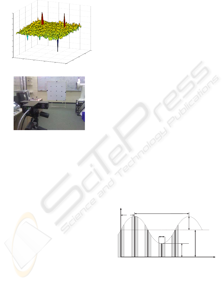
Figure 1: Range data (a) obtained for the PMD 3ks TOF

camera imaging a ﬂat board (b) pasted with nine low re-

ﬂectivity patches. The SNR

varies from 44.4db (forwhite

board) to 7.3db (for the low reﬂective patches). The varia-

tion associated with low SNR is clearly visible in the range

error seen in (a).

ill-conditioned inverse problem (Zhou et al., 2007).

The complexity and the degree of error due to min-

imization algorithms (Zheng and Chellappa, 1991),

and imaging conditions (Zhang et al., 1999) limits the

applicability of reﬂectance modelling of environment

in computer vision applications. Reliability of signal

strength and range data in the presence of unknown

reﬂectivity is a signiﬁcant challenge for TOF cameras

in real environments. To authors’ knowledge there is

little or no prior work to overcome TOF range mea-

surement error due to signal strength variation, inde-

pendent of scene reﬂectance.

This paper investigates the radiometric mod-

elling of TOF measurements and background light

sources by exploiting the dependencies between am-

plitude, intensity and range/phase measurements. We

consider statistical noise model of TOF measure-

ments, that along with radiometric properties of light

sources, and a Lambertian reﬂectance model enable

us derive a radiometric range model. Further in-depth

statistical analysis of parameters of this model is used

to formulate a radiometric range criterion. From this

criterion we can effectively evaluate pixel-by-pixel re-

liability of range measurement in TOF cameras that

is independent of scene reﬂectivity. For the purpose

of this conference paper, we restrict our attention to

the case of planar surfaces. The proposed reliability

criterion helps in evaluating and ﬁltering TOF range

measurements under various SNR conditions, a key

parameter for radiometric range criterion.

The paper is organized as follows: Section 2 de-

scribes TOF signal measurement, Section 3 provides

statistical models for the measurements, Section 4 de-

scribes a reﬂectance model from TOF camera per-

spective and Section 5 presents a radiometric range

model. In Section 6 we provide statistical analysis of

radiometric range model, and then go on to propose a

range pixel reliability criterion in Section 7. Section

8 presents experimental results of the implementation,

and a short conclusion follows.

2 TIME-OF-FLIGHT SIGNAL

MEASUREMENT

Time-of-Flight (TOF) sensors estimate distance to a

target using the time of ﬂight of a modulated in-

frared (IR) wave between the target and the cam-

era. The sensor illuminates/irradiates the scene with

a modulated signal of amplitude A (exitance) and re-

ceives back a signal (radiosity) after reﬂection from

the scene with background signal offset I

that in-

cludes non-modulated DC offset generated by TOF

camera as well as ambient light reﬂected from the

scene (see Figure 2).

There is a phase delay of the received modulated

signal proportional to the ratio of range on speed of

light of the observed point in the scene. The ampli-

time

= 20 MHz, T = 50 nsec

Signal strength

mod

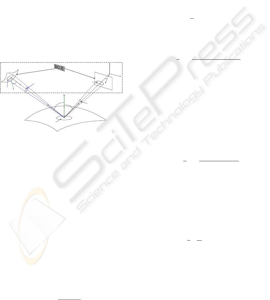
Figure 2: Received modulated signal in TOF camera. The

signal of modulated frequency f

mod

= 20Mhz with back-

ground illumination (exitance) I

, is sampled four times

. These measurements are used to calculate

amplitude A (1), phase ϕ (2) and intensity I (3).

tude and phase of a modulated signal can be extracted

by demodulating the incoming signal A = A

cos(ωt

VISAPP 2010 - International Conference on Computer Vision Theory and Applications

144

ϕ) + I; (t

= i ·

2ω

,i = 0,. ..3) (see Figure 2) by syn-

chronously sampling the received signal four times at

quarter wavelength intervals of the modulated source

frequency. The measured amplitude A, intensity I rep-

resenting the gray scale image and the phase of the

received signal are then respectively given by (Lange

and Seitz, 2001)

A :=

−A

)

+ (A

−A

)

(1)

ϕ := arctan

−A

. (2)

I :=

+ A

. (3)

With known phase ϕ, modulation frequency f

mod

and

precise knowledge of speed of light c, it is possible to

measure the un-ambiguous distance r from the cam-

era as

r := ϖϕ; where ϖ =

4π f

mod

. (4)

With a wavelength of λ =

mod

, this leads to a maxi-

mum possible unambiguous range of

. For the PMD

3k-S TOF, the modulation frequency is 20MHz and

the maximum unambigiuos range is 7.5m.

3 STATISTICAL NOISES

MODELS OF THE

MEASUREMENTS

It has been shown (Lange and Seitz, 2001) that pho-

ton shot noise effects the optical measurement process

and is the major statistical noise process in TOF de-

vices. In (Mufti and Mahony, 2009), statistical mod-

els for amplitude, phase and intensity were proposed

that model the achievable signal-to-noise ratio (SNR)

of the sensor device.

The statistical distribution of amplitude is a Rice

distribution given by

A ∼ Rice

I/2

, (5)

where

A denote the actual measurement obtained by

the TOF camera while A and I are the physical pa-

rameters of the model. The statistical distribution of

phase

ϕ is given by

Φ(

ϕ|A,ϕ,

I/2) =

2π

exp

−

1 +

√

cos(

ϕ −ϕ)

(

√

π)exp

cos

(

ϕ −ϕ)

1 + erf

A cos(

ϕ −ϕ)

√

´oi

, (6)

where erf(.) is the error function. Here Φ is a

marginal distribution obtained by integrating over the

joint distribution function of a complex version of the

received signal (Bonny et al., 1996). The range mea-

surement can be related to phase measurement based

on the model (4) as

ˇr = ϖ

ϕ. (7)

The statistical distribution for intensity is given by

(Mufti and Mahony, 2009)

I ∼ N (I,I/4). (8)

The measurements

ϕ, ˇr are thought of as the mea-

sured values of A,I,ϕ and r at pixel (x).

For a TOF camera a key performance parameter,

SNR is deﬁned as (Lange and Seitz, 2001; B

uttgen

et al., 2006; Mufti and Mahony, 2009)

SNR =

√

. (9)

In (Mufti and Mahony, 2009), the relationship of

phase with SNR has been shown by noting the fact

that although the phase distribution (6) is written with

dependence on three parameters (A, ϕ,

I/2), in fact

only the ratio,

√

I/2

, appears on the right hand side in

the deﬁnition of (6). Consequently the phase distribu-

tion can be re-written as

ϕ ∼ Φ

,ϕ,

√

= Φ

ϕ 1, ϕ,

SNR

. (10)

The model for SNR is a generic model for TOF

cameras (B

uttgen et al., 2006). In practice manufac-

turers vary the conﬁguration for customized designs

to improve performance in ways that do not funda-

mentally change the physics of the model but leads to

scaling effects that must be modelled. This process

for raw measurements is discussed in (Luan, 2001;

Mufti and Mahony, 2009) and is not further consid-

ered in this paper, although these effects must be un-

derstood to obtain experimental results.

We deﬁne a second key statistical factor for per-

formance measurement in TOF camera as signal-to-

offset ratio (SOR) of photon count. This ratio reﬂects

the total offset in the received signal with respect to

the amplitude of the modulated source and is given

SOR =

received signal amplitude

value of the background offset

. (11)

RADIOMETRIC RANGE IMAGE FILTERING FOR TIME-OF-FLIGHT CAMERAS

145

4 REFLECTANCE MODEL

The active signal of a TOF camera can be used for

measurement of amplitude A, intensity I, and range

r. These measurement parameters are not indepen-

dent but depend on the reﬂectance characteristics of

the scene. In order to develop reliability criteria for

TOF data it is necessary to provide background the-

ory for a reﬂectance model for time-of-ﬂight (TOF)

camera and understand the signal behavior in a radio-

metric framework.

A reﬂectance model gives a relationship for light

emitted and received between a source, a surface and

the observer or the camera image plane. We consider

a near-ﬁeld IR point source for the camera’s active

LED array and a far-ﬁeld source for background illu-

mination.

TOF camera

Transmitter and receiver in same housing

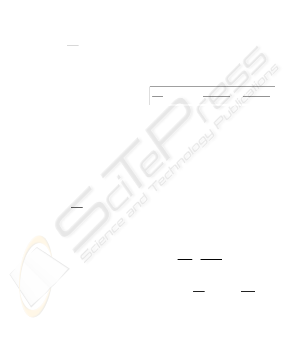
Figure 3: Geometry of reﬂectance model for Time-of-

Camera. Note that although the source and receiver of a

physical TOF camera are co-located, it is difﬁcult to pro-

vide a visualization of this geometry. Here the source is

shown separately to make is easier to see notation, however,

in practice the directional vectors r and x

are equal.

4.1 Reﬂectance Model for an IR Source

of TOF Camera

The primary source of illumination in TOF cameras

is an IR source that produces a modulated IR signal

offset by a non-modulated DC signal. The reﬂectance

model takes into account the modulated signal

represented by A(s) as well as the non-modulated DC

signal represented by I

(s).

Modulated IR Source. Let P be a Lambertian surface

in space with n

the normal to the each point p ∈ P

on the surface as shown in Figure 3. Let a modulating

IR point source S is irradiating the surface P then dω

denote the solid angle of dA

seen from point p. Then

dω =

cosθ

, (12)

where θ

is the angle between the normal to the

source point s ∈ S and the ray of the modulated IR

signal reaching point p, and r is the distance between

source and the point p. Following the laws of radiom-

etry (Sillion and Puech, 1994) the amplitude of total

radiance A(p) (called radiosity) leaving point p due

to illumination by the modulated signal A(s) is pro-

portional to the diffuse reﬂectance or albedo ρ(p) and

the integral of irradiance over all the possible incom-

ing directions in a hemisphere, Ω, scaled by the cosine

of arrival angle θ

(Ma et al., 2003) (p. 68)

A(p) =

Ω

ρ(p)A(s)cos θ

dω. (13)

By substituting (12) into (13) and changing the do-

main of integration to the surface, S, of the source

(Forsyth and Ponce, 2003) (p. 77), one has

A(p) =

ρ(p)

A(s)cos θ

cosθ

. (14)

An active TOF camera senses the received modulated

IR signal within its ﬁeld of view and all the points

on surface illuminated by the camera can observe the

same source. In the present analysis, the LED point

sources of the camera are part of the compact IR ar-

ray of the TOF camera, and can be approximated by

a single virtual modulated point source (Forsyth and

Ponce, 2003, p. 78) with the center of illumination

aligned with the center of projection and the optical

axis of the camera (Kuhnert and Stommel, 2006). In

this case, the integration (14) can be re-written as a

function of the exitance of a single point source as

A(p) :=

ρ(p)

A(s)cos θ

cosθ

. (15)

Using the thin lens assumption, irradiance on an

image plane can be expressed by measuring the ra-

diosity along the direction x that depends on the ge-

ometry of the lens capturing the light (Ma et al., 2003,

p. 48) as

A(x) = ϒA(p). (16)

Here ϒ is the lens collection representing irradiance

fall-off with cosine-fourth law (Horn, 1986) (p. 208)

ϒ =

cos

, (17)

where d is the diameter of the lens, f

is the focal

length of the lens and θ

is the angle of the ray from

the principle axis.

Non-modulated IR Source. The TOF camera

IR source produces a DC signal from the same IR

source LEDs. This signal will have the same re-

ﬂectance model as has been derived for the modulated

VISAPP 2010 - International Conference on Computer Vision Theory and Applications

146

IR source (see (15)). One has

(p) :=

ρ(p)

(s)cos θ

cosθ

, (18)

where the received signal I

(x) is given by

(x) = ϒI

(p). (19)

The effect of this signal is an added offset to the mod-

ulated signal for better illumination of the scene.

4.2 Reﬂectance Model for Background

Illumination

We also consider the background illumination of

the scene due to ambient light in TOF camera. In

computer vision (Alldrin et al., 2008) and computer

graphics (Cook and Torrance, 1982), a single view

point source of local shading model and an ambient

illumination model is generally preferred and we

would restrict our attention to these two models of

background illumination.

Ambient Background Illumination. Consider

an ambient background illumination of the scene i.e

an illumination that is constant for the environment

and produces a diffuse uniform lighting over the

object (Foley et al., 1997) (p. 723). Let I

be the in-

tensity (called exitance) of the ambient illumination,

then the received intensity I

(p) from a point p is

expressed as

(p) =

ρ(p)I

, (20)

where ρ, is the ambient reﬂection coefﬁcient of a sur-

face. The irradiance on the image plane is given by

(x) = ϒI

(p). (21)

Far Field Background Illumination. For real envi-

ronments we also consider far-ﬁeld point sources. For

a point source that is far away as compared to the area

of the target surface, the exitance does not depend on

the distance from the source or the direction in which

the light is emitted (Forsyth and Ponce, 2003) (p. 76).

The radiosity of point p due a point source q ∈ Q,

deﬁned as I

(p), can be obtained by integrating each

of the sources as

(p) =

ρ(p)

(q)cos θ

, (22)

where θ

is the angle between normal to the surface

point p and the source point q, ρ(p) is the surface

albedo at point p and dA

is the inﬁnitesimal area of

a source Q. Considering a single IR far-ﬁeld back-

ground point source of illumination, the radiosity per-

ceived by TOF image plane due to this IR source is

given as

(x) = ϒI

(p). (23)

where

(p) =

ρ(p)I

(q)cos θ

. (24)

5 RADIOMETRIC RANGE

MODEL

In Section 4, we derived the reﬂectance model for the

signal received by TOF camera. The perceived ra-

diosity for each pixel x is highly dependent on the

unknown diffuse reﬂectance ρ(p) (see (15), (18), (20)

and (24)). The value of this parameter ranges between

0 and 1. The received signal can have large ﬂuctua-

tions corresponding to a different reﬂectivity of differ-

ent points p in the scene observed at pixel x. As a con-

sequence, there is a signiﬁcant deviation in statistical

distribution of distance measurements for TOF cam-

era for different reﬂective surfaces (Lindner and Kolb,

2007; Mufti and Mahony, 2009). The received signal

obtained after reﬂection from object with very low re-

ﬂectivity will lie in a region of low SNR. In 2D cam-

eras the only available measurement is intensity and

photometric stereo techniques are used to estimate re-

ﬂectivity from multiple images or light orientations

to solve the associated under-determined system. A

TOF camera, however, measures amplitude, intensity

and phase. Hence, it is possible to create a uniﬁed

reﬂectance model based on all the available measure-

ment parameters that is robust against limitation of

unknown reﬂectivity.

From the basic principles of TOF camera signals

shown in Figure 1, we know that the intensity compo-

nent of TOF carries information for both, amplitude

of the modulated signal and the background offset I

Thus, we can represent the mean offset represented by

intensity of TOF cameras as

I := A + I

. (25)

The background offset I

is composed of DC offset

due to TOF camera I

and background illumination I

and I

depending upon the environment where TOF

camera is operating. One has

= I

+ I

. (26)

Indexing the point p in the scene by the TOF receiv-

ing pixel x and dividing (25) by A(x) and substituting

(26), one obtains

I(x)

A(x)

= 1 +

(x)

A(x)

(x)

A(x)

(x)

A(x)

. (27)

RADIOMETRIC RANGE IMAGE FILTERING FOR TIME-OF-FLIGHT CAMERAS

147

Using the local shading model for IR signal and the

background illumination of point sources (16), (19),

(21) and (23), one can re-write (27) as

I(x)

A(x)

= 1 +

(s)

A(s)

(x)

A(s)cosθ

cosθ

(q)cosθ

(x)

A(s)cosθ

cosθ

(28)

where θ

:= θ

(x) is a function of pixel.

The ratio of background ambient light I

to mod-

ulated TOF IR source A(s) can be deﬁned as

A(s)

. (29)

Observe that κ

does not depend upon scene or cam-

era geometry and hence is a constant parameter over

the full image array. Similarly, deﬁne

(q)

A(s)

, (30)

as the ratio of far-ﬁeld illumination and the TOF IR

source. The parameter κ

is once again a constant pa-

rameter independent of scene or pixel coordinates. Fi-

nally we deﬁne κ

as the ratio of TOF non-modulated

IR source I

(s) and TOF modulated IR source A(s)

(s)

A(s)

, (31)

Since the two sources of illumination originate from

the same IR LED source, any surface in the scene

will receive same amount of modulated and non-

modulated TOF IR source due to identical angle of

illumination. Thus we can redeﬁne (31)

(x) :=

(

)

A(x)

. (32)

where κ

(x) is function of a pixel x ∈R

and is a cam-

era based pixel parameter for an entire image. In the-

ory κ

(x) = κ

for all x that varies with the integra-

tion time. However, in practice slight variation in the

CMOS circuitry causes pixel variation in κ

(x) and is

modelled using calibration techniques documented in

Section 6.

The parameters (κ

,κ

) are constant over the im-

age plane. For any surface patch

, it is possible to

numerically compute an estimate of the angle θ

(x)

from the set of range measurements r(x

) associated

with that patch based on an estimate of the normal

vector to the surface (Pulli and Pietikainen, 1993;

Klasing et al., 2009; Ye and Hedge, 2009). For the

far ﬁeld source we add two parameters (θ

,θ

) that

describe its azimuth and elevation with respect to the

camera frame. Given the estimate θ

,θ

then it is

The surface patch must be sufﬁciently large to be im-

aged by a small window of pixels.

also straightforward to compute θ

(x). We think of

these angles as functions of range data from pixels

corresponding to a local surface around a point in the

image. That is, denoting the local neighbourhood of x

by {x

}

i=1

used in the calculation of normal to x, one

has

(x) := F

[r(x

),··· ,r(x

)] (33)

(x) := F

[r(x

),··· ,r(x

),θ

,θ

]. (34)

Although the present spatial resolution of TOF cam-

eras have signiﬁcant limitations, it is clear that future

technology will lead to TOF cameras with potentially

much higher resolution, making this process highly

effective.

Thus, using the parameters (κ

,κ

,θ

) of

sources one obtains a radiometric relationship as

I(x)

A(x)

= 1 + κ

(x) + κ

(x)

cosθ

+ κ

cosθ

(x)

cosθ

(35)

The above radiometric relationship is independent of

reﬂectivity ρ(p) and relate the measurable variables

A,I,r to constant parameters κ

,κ

and θ

,θ

5.1 Radiometric Range Model for

Planar Case

In this paper, we will only consider the case of ra-

diometric range model for planar surfaces using (35).

Consider the case of a single planar surface in the ﬁeld

of view of TOF camera. Over this single surface it can

be easily seen that θ

is constant while θ

is nearly

constant for a small ﬁeld of view of TOF optical sen-

sor over the surface. As a result several parameters

can be combined into a single constant. We propose

an approximate model

I(x)

A(x)

= 1 + κ

(x) + κ

(x)

cosθ

, (36)

where

cosθ

= constant. (37)

As a consequence of (37), a pixel measurement of κ

is given by

(x) =

I(x)

A(x)

−κ

(x) −1

cosθ

(x)

. (38)

We will use κ

(x) as a radiometric criterion for range

reliability.

In practice the measurement of κ

(x) is a noisy

process due to noise in the statistical distribution of

measurement obtained. In the next section we provide

a detailed analysis of statistical distributions of κ

(x)

and parameters associated with it due to the noise in

the measurement process.

VISAPP 2010 - International Conference on Computer Vision Theory and Applications

148

6 STATISTICAL DISTRIBUTION

(x)

We have seen that κ

is a function of constant sources

(camera source and the background source of illumi-

nation) that cannot be directly measured in practice.

The relationship (38) provides a mean to measure κ

in practice. A statistical analysis of the measurement

of κ

(x) in this section will provide a signiﬁcant in-

sight into radiometric range model for the planar case.

Consider a pixel x in the TOF image array and de-

ﬁne the measurement

(x) as

(x) :=

−

−1

cosθ

ˇr

, (39)

where

is an estimate of camera based parameter for

an entire image. A

(x) is complex statistical distri-

bution composed of ratio of different distribution and

as such a closed form analytic solution is not possible.

However, based on the distributions of measurements

I, ˇr and the estimate of

, we can represent the sta-

tistical distribution of

(x) in terms of independent

parameters. The statistical distributions of

I and ˇr

have been discussed in Section 3.

The ratio of modulated and non-modulated IR

source of TOF camera, κ

(x), is ﬁxed for each pixel

and is determined as a pre-processing step in TOF ra-

diometric range estimation. The estimation of κ

(x)

deﬁned as

is a measurement process over a large

data set. For sufﬁcient samples central limit theorem

ensures that,

∼ N

(x),

[κ

(x)]

. (40)

By knowing the distribution of dependent param-

eters we can now show that

(x) is sampled from

a distribution with three pixel based independent

parameters SNR, SOR and κ

. The two parameters κ

and θ

are camera parameters that can be calibrated in

the initial setup of the camera and are not considered

parameters of the distribution.

Lemma 1:

(x) Distribution Parameters.

Assume the camera parameters κ

(x) and θ

are

known and

A(x), ˇr(x),

I(x) are given by (5),(7) and

(8). Then the measurement

(x) =

I(x)

A(x)

−κ

(x) −1

cosθ

ˇr

(x)

, (41)

can be modelled as a random variable with distri-

bution depending on three independent parameters

SNR (9), SOR (11) and κ

(37).

Proof: Recall that A(x),I(x) and r(x) are the

underlying radiometric parameters of the ideal re-

ceived signal based on noise free radiometric model.

For ease of notation we drop the (x) dependence such

that A = A(x), I = I(x). Using the deﬁnition of SOR

(11) and (26), one can write

SOR

+ I

. (42)

Using (37), one has

A(s)cos θ

+ I

(q)cos θ

). (43)

Deﬁne new scaled measurement

A :=

A/A and

I :=

I/A then it is straight forward to verify from (5) and

(8) that

A =

∼ Rice

√

= Rice

SNR

(44)

I =

∼ N

+ A

= N

1 + SOR

SOR

2 ·SNR

(45)

Using the radiometric model (16) for the true

range r, one has

ϒρ(p)

A(s)cos θ

cosθ

ϒρ(p)

A(s)cos θ

cosθ

+ I

(q)cos θ

)

+ I

(q)cos θ

)

= cosθ

A(s)cos θ

+ I

(q)cos θ

+ I

. (46)

Substituting (42) and (43), we obtain

cosθ

SOR

−κ

. (47)

As a consequence of (4) one can write the true phase

ϕ :=

cosθ

SOR

−κ

(48)

Hence, using (7) and (10) we have shown

ˇr ∼

ˇr

cosθ

SOR

−κ

SNR

. (49)

This shows that ˇr is a random variable with param-

eters SNR, SOR and κ

. From (41), using (44),(45)

and (49) one has

(x) =

−κ

−1

cosθ

ˇr

. (50)

Thus, the expression for

(x) is a function of random

variables

I and ˇr. The random variables depend in

RADIOMETRIC RANGE IMAGE FILTERING FOR TIME-OF-FLIGHT CAMERAS

149

turn on the parameters SNR, SOR and κ

(44),(45)

and (49). Consequently,

(x) is a random variable

depending on parameters SNR, SOR and κ

Let f

denote the distribution function for

(x). That

(x) ∼ f

(

(x)|SNR,SOR,κ

). (51)

The SNR is the dominant parameter of

(x) distribu-

tion due to the shot noise associated with Poisson ar-

rival process of photons of TOF signal and effects the

spread or tail of

(x) distribution. The parameters

SOR and κ

effect the mean value of the distribution.

0 10 20 30 40 50

0.02

0.04

0.06

0.08

0.1

0.12

Probaility density fucntion P(˘κ

)

˘κ

MC simulation

PMD data

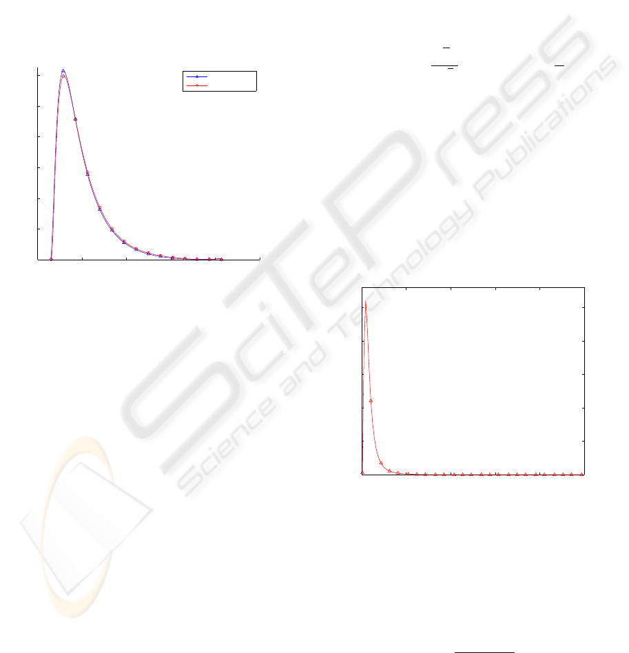
Figure 4:

(x) Plot for Monte Carlo simulation and

real data from PMD camera (SNR

=12.14db, SOR

38.61db, κ

=8.39).

It appears to be extremely difﬁcult to derive an an-

alytic expression for the distribution of

(x). We

verify the model using Mote Carlo simulation with

model parameters A,I and ϕ to plot

(x) distribu-

tions (with parameters SNR, SOR, and κ

). A low

SNR case is plotted in Figure 4. The measured range

variation for this case is between 1.95m to 3.82m. The

simulation data matches with the experimental data,

conﬁrming the validity of the proposed model param-

eters.

7 RADIOMETRIC RANGE

CRITERION FOR PIXEL

RELIABILITY

In this Section, we propose an algorithm for radio-

metric range ﬁltering. The statistical analysis of

(x)

distribution (51) lead us to formulate a reliability cri-

teria based on a statistical test for

(x). That is given

estimates

SNR(x),

SOR(x) and

(x) of parameters

SNR, SOR and κ

at pixel x, let α > 0 signiﬁcance

level, choose m(x) such that

(

(x) < m(x))|

SNR(x),

SOR(x),

(x)

= α,

(52)

where

∞

m(x)

[

κ|

SNR(x),

SOR(x),

(x)]d

κ = α. (53)

Then,

(x) is accepted if

(x) < m(x).

Consider a single frame of data and note that the

estimates of

SNR(x) and

SOR(x) can be computed

pixel-by-pixel as

SNR(x) =

√

;

SOR(x) =

, (54)

where

is the measured background offset. In addi-

tion, it is necessary to compute the estimate of

(x)

at pixel x. Based on the assumption of a ﬂat surface

the true value of κ

(x) will only deviate from a con-

stant due to viewing angle of the surface θ

. This an-

gle is approximately constant for small ﬁeld of view

cameras. Therefore, we approximate κ

(x) ≈ κ

over

pixels of the planar surface. Moreover, we ﬁnd in

practice that the SNR and SOR over a single planar

surface are comparable and we can make an estimate

of κ

based on average statistics of this data set.

0 20 40 60 80 100

0.05

0.1

0.15

0.2

0.25

˘κ

Relative contribution of ˘κ

Figure 5: Normalized histogram of

(x) of a surface. Pix-

els with

(x) → ∞ (due to amplitude and phase) have been

scaled down to ﬁnite values.

A typical normalized histogram of

(x) for a sin-

gle frame of a planar surface is shown in Figure 5.

The heavy tail is associated with noisy data. We pro-

pose a pragmatic approach (a practical estimator) for

using the harmonic mean

∑

o(x)

(55)

It is reasonable to use the harmonic mean (Bodek,

1974) due to the fact that each individual

(x) is a

VISAPP 2010 - International Conference on Computer Vision Theory and Applications

150

ratio distribution with different SNRs of the received

signal measured in TOF camera and the error mea-

surements of

(x) in denominator being greater than

that of a numerator.

The statistical test (52) can be applied to all pix-

els drawn from a planar surface. The parameters

SNR,

SOR,

estimated from the same data that is

then used in the test, however, the slight dependence

introduced is not believed to effect the overall valid-

ity of the test signiﬁcantly if there are enough pixels

in the given observed surface (typically a 5×5) patch.

8 EXPERIMENTS AND RESULTS

We perform experiments in an indoor environment

where a TOF camera is placed conveniently at a dis-

tance of 3 meters from a ﬂat white board while the

wall is about 6 meters from the camera as illustrated

in Figure 6. In addition there are various other objects

and lab equipment within the ﬁeld of view of camera.

These objects offer different reﬂectivity and provide

a wide variety of characteristics for the experiments

undertaken. Our PMD 3k-S(PMD, 2002) TOF cam-

era provides 48×64 pixel resolution with a ﬁeld of

view of 33.4

◦

×43.6

◦

Figure 6: Picture taken from a normal 2D camera for a tri-

pod mounted TOF camera setup.

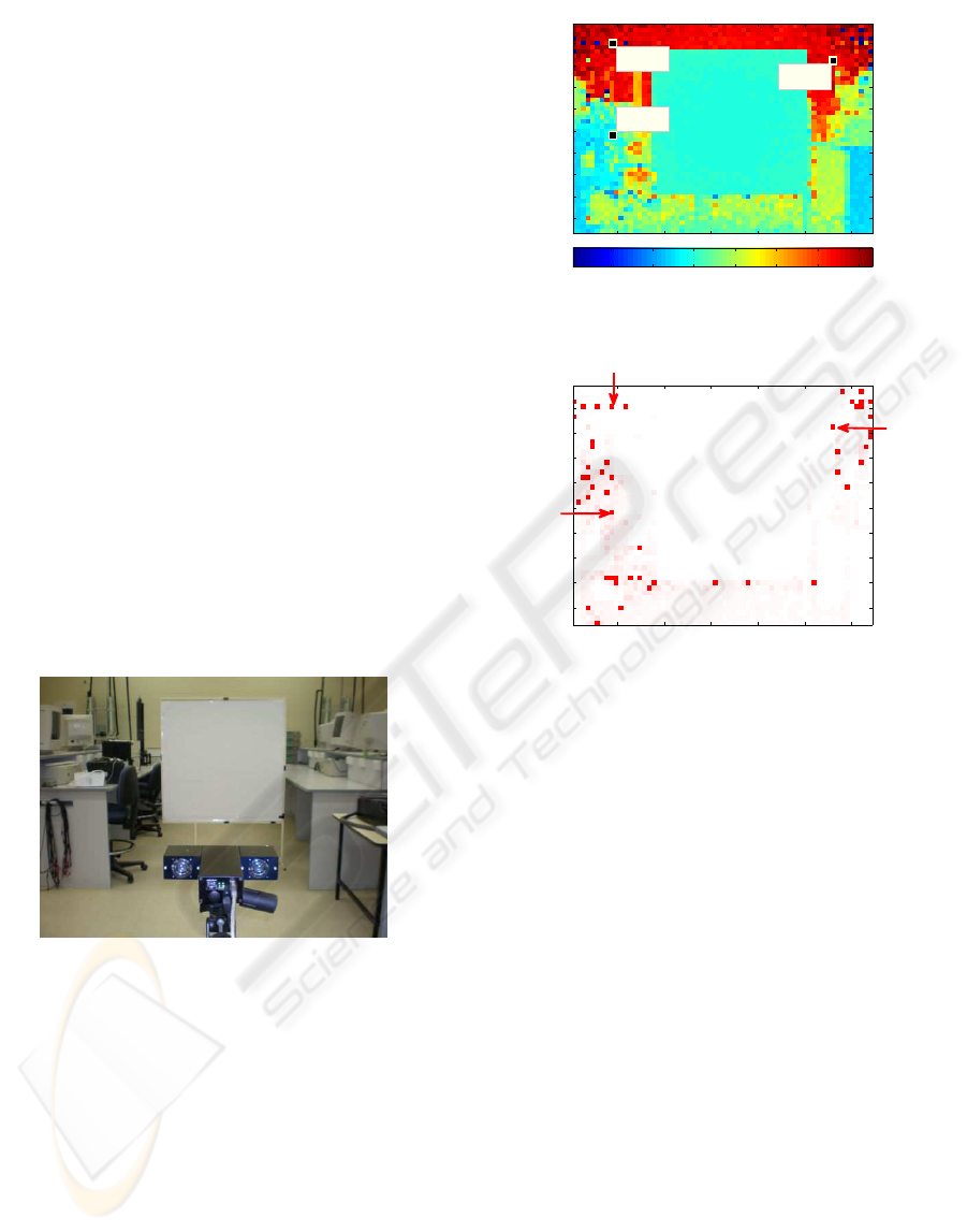
The algorithm is applied to an entire frame and

(x) distribution is plotted for a planar surface (a

wall) (see Figure 5). The ﬁnal range data as a function

(x) is obtained after applying the range image

ﬁltering criterion (52) to the entire frame including

planar surface as shown in Figure 8.

The ﬁnal6data after ﬁltering is consistent with a

reliable measurement of range values. It is quite clear

that

(x) value is almost consistent for the entire

range (0-7.5 meters) of the camera with noisy data

pixels (see Figure 7) showing a variation in

(x) val-

ues as shown in Figure 8. The algorithm is neither

effected by the distance of the object from the cam-

era (within camera range) nor the reﬂectively/surface

X: 9 Y: 5

Range: 1.014

X: 56 Y: 9

Range: 0.077

X: 9 Y: 26

Range: 1.951

10 20 30 40 50 60

1 2 3 4 5 6 7

meters

Figure 7: Range image plot of a PMD TOF camera with

three marked noisy (in-correct) range pixels.

10 20 30 40 50 60

Figure 8: Filtered

(x) plot with regions of consistent

and noisy pixels shown in red color. Three pixels marked

with arrows relate to marked noisy range pixels in Figure 7.

texture for wide range of integration times and SNR

conditions compared to other image algorithms that

are otherwise susceptible to surface conditions. It has

been observed that in real environments the planar

model works extremely well even for non-planar sur-

faces and is robust enough for reliable range measure-

ments. Since the applied algorithm can ﬁlter the entire

frame, the algorithm is quite efﬁcient and effective for

TOF based applications.

9 CONCLUSIONS

The use of Time-of-ﬂight (TOF) cameras is increasing

in various applicati6ns ranging from medical to auto-

motive. TOF manufacturer companies are progress-

ing rapidly to increase the resolution and range of the

camera. However, the range pixel reliability has not

been addressed effectively in the literature. The use of

radiometric model for all the available measurement

parameters helps in formulating a robust range relia-

bility criterion that is independent of scene reﬂectivity

and will make a substantial difference to how range

pixel reliability is classiﬁed.

RADIOMETRIC RANGE IMAGE FILTERING FOR TIME-OF-FLIGHT CAMERAS

151

ACKNOWLEDGEMENTS

This work is supported by Seeing Machines Ltd. and

the Commonwealth of Australia, through the Coop-

erative Research Centre for Advanced Automotive

Technology.

REFERENCES

Alldrin, N., Zickler, T., and Kriegman, D. (2008). Pho-

tometric stereo with non-parametric and spatially-

varying reﬂectance. In Proc. IEEE Conference

on Computer Vision and Pattern Recognition CVPR

2008, pages 1–8.

Bodek, A. (1974). The mean of several quotients of two

measured variables. SLAC Technical Note.

Bonny, J.-M., Renou, J.-P., and Zanca, M. (1996). Opti-

mal measurement of magnitude and phase from MR

data. Journal of Magnetic of Resonance, Series B,

113(2):136–144.

uttgen, B., Lustenberger, F., and Seitz, P. (2006). Demod-

ulation pixel based on static drift ﬁelds. IEEE Trans.

Electron Devices, 53(11):2741–2747.

Cook, R. L. and Torrance, K. E. (1982). A reﬂectance

model for computer graphics. ACM. Trans. on Graph-

ics, 1(1):7–24.

Fardi, B., Dousa, J., Wanielik, G., Elias, B., and Barke, A.

(2006). Obstacle detection and pedestrian recognition

using a 3D PMD camera. In Proc. IEEE Intell. Vehi-

cles Symp., pages 225–230.

Foley, J. D., Da, A. v., Feiner, S. K., and Hughes, J. F.

(1997). Computer Graphics: Principles and Prac-

tices. Addisin-Wesley Publishing Company, Inc.

Forsyth, D. A. and Ponce, J. (2003). Computer Vision: A

Modern Approach. Prentice Hall.

Horn, B. (1986). Robot Vision. The MIT Press.

Horn, B. K. P. (1977). Image intensity understanding. Arti-

ﬁcial Intelligence, 8(2):201–231.

Kahlmann, T., Remondino, F., and Guillaume, S. (2007).

Range imaging technology: new developments and

applications for people identiﬁcation and tracking. In

Proc. SPIE-IS&T Electronic Imaging, volume 6491,

San Jose, CA, USA.

Kahlmann, T., Remondino, F., and Ingensand, H. (2006).

Calibration for increased accuracy of the range imag-

ing camera SwissRanger. In Proc. International

Archives of Photgrammetry, Remote Sensing and Spa-

tial Information Sciences, ISPRS Commission V Sym-

posium, volume XXXVI, pages 136–141.

Klasing, K., Althoff, D.,Wollherr, D., and Buss, M. 2009

Comparison of surface normal estimation methods for

range sensing applications. In Proc. IEEE Interna-

tional Conference on Robotics and Automation ICRA

09, pages 32063211.

Kuhnert, K.-D. and Stommel, M. (2006). Fusion of stereo-

camera and PMD-camera data for real-time suited

precise 3D environment reconstruction. In Proc.

IEEE/RSJ Int. Conf. Intell. Robot. Systs.

Lange, R. and Seitz, P. (2001). Solid-state time-of-ﬂight

range camera. IEEE J. Quantum Electron., 37:390–

397.

Lindner, M. and Kolb, A. (2006). Lateral and depth calibra-

tion of PMD-distance sensors. In Proc. International

Symposium on Visual Computing (ISVC06), volume 2,

pages 524–533. Springer.

Lindner, M. and Kolb, A. (2007). Calibration of the

intensity-related distance error of the PMD TOF-

camera. In Proc. SPIE, Intelligent Robots and Com-

puter Vision XXV: Algorithms, Techniques, and Active

Vision, volume 6764.

Luan, X. (2001). Experimental Investigation of Photonic

Mixer Device and Development of TOF 3D Ranging

Systems Based on PMD Technology. PhD thesis, De-

partment of Electrical Engineering and Computer Sci-

ence at University Of Siegen.

Ma, Y., Soatto, S., Ko

seck

a, J., and Sastry, S. S. (2003).

An Inviation to 3-D Vision: From Images to Geomtric

Models. Springer Verlag. Ch. 2.

Meier, E. and Ade, F. (1997). Tracking cars in range image

sequnces. In Proc. IEEE Int. Conf. Intell. Trans. Systs.,

pages 105–110.

Moller, T., Kraft, H., Frey, J., Albrecht, M., and Lange,

R. (2005). Robust 3D measurement with PMD sen-

sors. In Proc. 1st Range Imaging Research Day, ETH

Zurich, Zurich, Switzerland.

Mufti, F. and Mahony, R. (2009). Statistical analysis of

measurement processes for time-of-ﬂight cameras. In

Proc. SPIE Videometrics, Range Imaging, and Appli-

cations X, volume 7447-21.

PMD (2002). PMD tech. http://www.pmdtec.com.

Pulli, K. and Pietikainen, M. (1993). Range image segmen-

tation based on decomposition of surface normals. In

Proc. 8th Scandinavian Conference on Image Analy-

sis, pages 893–899.

Radmer, J., Fuste, P. M., Schmidt, H., and Kruger, J. (2008).

Incident light related distance error study and cali-

bration of the PMD-range imaging camera. In IEEE

Conf.Computer Vision and Pattern Recognition Work-

shops, 2008, pages 16.

Sillion, F. X. and Puech, C. (1994). Radiosity and Global

Illumination. Morgan Kaufmann.

Ye, C. and Hegde, G.-P. M. (2009). Robust edge extrac-

tion for SwissRanger SR-3000 range images. In Proc.

IEEE International Conference on Robotics and Au-

tomation ICRA09, pages 24372442.

Zhang, R., Tsai, P.-S., Cryer, J., and Shah, M. (1999). Shape

from shading: A survey. IEEE Trans. Pattern Anal.

Mach. Intell., 25(11):1416–1421.

Zheng, Q. and Chellappa, R. (1991). Estimation of illu-

mination direction, albedo, and shape from shading.

IEEE Trans. Pattern Anal. Mach. Intell., 13(7):680–

702.

Zhou, S., Aggarwal, G., Chellappa, R., and Jacobs, D.

(2007). Appearance characterization of linear lam-

bertian objects, generalized photometric stereo, and

illumination-invariant face recognition. IEEE Trans.

Pattern Anal. Mach. Intell., 29(2):230–245.

VISAPP 2010 - International Conference on Computer Vision Theory and Applications

152