
SCENE CLASSIFICATION USING SPATIAL RELATIONSHIP
BETWEEN LOCAL POSTERIOR PROBABILITIES
Tetsu Matsukawa
†
and Takio Kurita
‡
†
Department of Computer Science, University of Tsukuba, Tennodai 1-1-1 Tsukuba, Japan
‡
National Institute of Advanced Industrial Science and Technology (AIST), Umezono 1-1-1 Tsukuba, Japan
Keywords:
Scene classification, Higher order local autocorrelation features, Bag-of-features, Posterior probability image.
Abstract:
This paper presents scene classification methods using spatial relationship between local posterior probabilities
of each category. Recently, the authors proposed the probability higher-order local autocorrelations (PHLAC)
feature. This method uses autocorrelations of local posterior probabilities to capture spatial distributions of
local posterior probabilities of a category. Although PHLAC achieves good recognition accuracies for scene
classification, we can improve the performance further by using crosscorrelation between categories. We
extend PHLAC features to crosscorrelations of posterior probabilities of other categories. Also, we introduce
the subtraction operator for describing another spatial relationship of local posterior probabilities, and present
vertical/horizontal mask patterns for the spatial layout of auto/crosscorrelations. Since the combination of
category index is large, we compress the proposed features by two-dimensional principal component analysis.
We confirmed the effectiveness of the proposed methods using Scene-15 dataset, and our method exhibited
competitive performances to recent methods without using spatial grid informations and even using linear
classifiers.
1 INTRODUCTION
Scene classification technologies have many possi-
ble applications such as content-based image retrieval
(Vogel and Schiele, 2007) and also can be used as a
context for object recognition (Torralba, 2003). Until
now, many researchers have tackled this problem.
The most commonly used approach to scene clas-
sification is the approach that uses holistic or local
statistics of local features. Especially, the spatial
pyramid matching that uses bag-of-features on spatial
grids showed excellent classification performances in
scene classifications(Lazebnik et al., 2006). How-
ever, such spatial grided local statistics is weak for
spatial misalignment. Another alternative approach is
the spatial relationship of local features (Yao et al.,
2009). If we use the spatial relationship histogram
without spatial griding, this representation may be ro-
bust against spatial misalignment. In this paper, we
realize the spatial relationship of local regions by us-
ing feature extractions on posterior probability im-
ages. A posterior probability image is the image in
which each pixel shows the confidence of one of the
given categories. Although the image feature that fo-
cused on posterior probability has not been a standard
technique for scene classification so far, we focus on
the feature of posterior probability images by two rea-
sons as follows. a): One drawback of the spatial rela-
tionship of local features is the problem that possible
combination of visual codebook is very large. There-
fore, it was required to select distinguish codebook
sets (e.g. A priori mining algorithm in (Yao et al.,
2009)). b): Synonymy codebook(Zheng et al., 2008)
that has similar posterior probabilities of category is
existed, that may considered as redundant represen-
tations of local features. By using the relationship
of local posterior probabilities, such problems can be
handled.
Recently, as the features on posterior proba-
bility images, the authors proposed the probabil-
ity higher-order local autocorrelations (PHLAC) fea-
ture(Matsukawa and Kurita, 2009). This method is
designed by using higher order local autocorrelations
(HLAC) features (Otsu and Kurita, 1988) of cate-
gory posterior probability images. Although PHLAC
can capture spatial and semantic informations of im-
ages, the autocorrelation was restricted to the pos-
terior probabilities of a single class in the previous
study.
325
Matsukawa T. and Kurita T. (2010).
SCENE CLASSIFICATION USING SPATIAL RELATIONSHIP BETWEEN LOCAL POSTERIOR PROBABILITIES.
In Proceedings of the International Conference on Computer Vision Theory and Applications, pages 325-332
DOI: 10.5220/0002819903250332
Copyright
c
SciTePress

Figure 1: Proposed scene classification approach.
The crosscorrelation between posterior proba-
bility images of other categories might capture
richer informations for scene classification. In this
paper, we extend PHLAC features to categorical
auto/crosscorrelations. Also, we introduce subtrac-
tion operator for describing another spatial relation-
ship of local posterior probabilities. Since the com-
bination of category index is large, we compress the
proposed features by two-dimensional principal com-
ponent analysis(2DPCA) (Yang et al., 2004). Finally,
the proposed scene classification method becomes as
shown in Figure 1. The proposed method is effec-
tive for scene classification problems even using lin-
ear classifiers.
2 RELATED WORK
There are some approaches for scene classification;
classification with features on spatial domain (Ren-
ninger and Malik, 2004; Battiato et al., 2009; Szum-
mer and Picard, 1998; Gorkani and Picard, 1994),
and features on frequency domain(Oliva and Tor-
ralba, 2001; Torralba and Oliva, 2003; Farinella et al.,
2008; Ladret and Gue’rin-Dugue’, 2001). In scene
classification in spatial domain, a scene is repre-
sented as different forms such as histogram of visual
words(Lazebnik et al., 2006), textons(Battiato et al.,
2009), semantic concepts(Vogel and Schiele, 2007),
scene prototypes(Quattoni and Torralba, 2009) and so
on. Our motivation is to improve classification ac-
curacies of scene classification in spatial domain. To
this end, we focus on features on posterior probability
images (semantic information).
Rasiwasia et al. proposed a semantic feature rep-
resentation by using the bag-of-featuresmethod based
on the Gaussian mixture model (Rasiwasia and Vas-
concelos, 2008). In their study, each feature vector in-
dicated the probability of each class label, and they re-
fer to this type of scene labeling as casual annotation.
Using this feature, they could achieve high classifica-
tion accuracies with low feature dimensions. Meth-
ods that provide posterior probabilities to a codebook
have also been proposed (Shotton et al., 2008). How-
ever, these methods do not employ the spatial rela-
tionship of local regions. Recently, pixel(region) wise
scene annotation methods by predetermined concepts
(e.g. sky, road, tree) are researched by many authors
(Bosch et al., 2007). By combining their methods
to our methods, total scene categories (e.g. suburb,
coast, mountain) can be recognized. Vogel et al. clas-
sified local regions to semantic concepts by classi-
fiers and classified total scene categories using his-
togram representations of local concepts (Vogel and
Schiele, 2007). A similar method to PHLAC that
uses local autocorrelations of similarity of category
subspaces constructed by Kernel PCA was recently
proposed(Hotta, 2009). However, this method also
doesn’t use crosscorrelation between different cate-
gory subspaces.
3 PHLAC FEATURES
3.1 Posterior Probability Image
Let I be an image region, and r= (x, y)
t
be a posi-
tion vector in I. The image patches whose center is
r
k
are quantized to M codebooks {V
1
,...,V
M
} by local
feature extractions and the vector quantization algo-
rithm VQ(r
k
) ∈ {1,...,M}. These steps are the same as
that of the standard bag-of-featuresmethod (Lazebnik
et al., 2006). Posterior probability P(c|V
m
) of the cat-
egory c ∈ {1, ...,C} is calculated to each codebookV
m
using image patches on the training images. Several
forms of estimating the posterior probability can be
used. In this study, the posterior probability is esti-
mated by using Bayes’ theorem as follows.
P(c|V
m
) =
P(V
m
|c)P(c)
P(V
m
)
=
P(V
m
|c)P(c)
∑
C
c=1
P(V
m
|c)P(c)
, (1)
where P(c) = 1/C, P(V
m
)= (# of V
m
)/(# of all
patches), P(V
m
|c) = (# of class c ∧ V
m
)/(# of class
c patches). Here, P(c) is a common constant and here
is set to 1.
In this study, the grid sampling of local features
(Lazebnik et al., 2006) is carried out at pixel interval
of p for simplicity. We denote the set of sample points
as I
p
and the map of posterior probability of the code-
book of each local region as a posterior probability
image. Examples of posterior probability images are
shown in Figure 2. White color represents the high
probability. Note that the forest like regions appear
in the vegetations of each image, and the flat regions
such as sky have high probability of highway. In these
way, each semantic region can be roughly character-
ized through class label.
VISAPP 2010 - International Conference on Computer Vision Theory and Applications
326
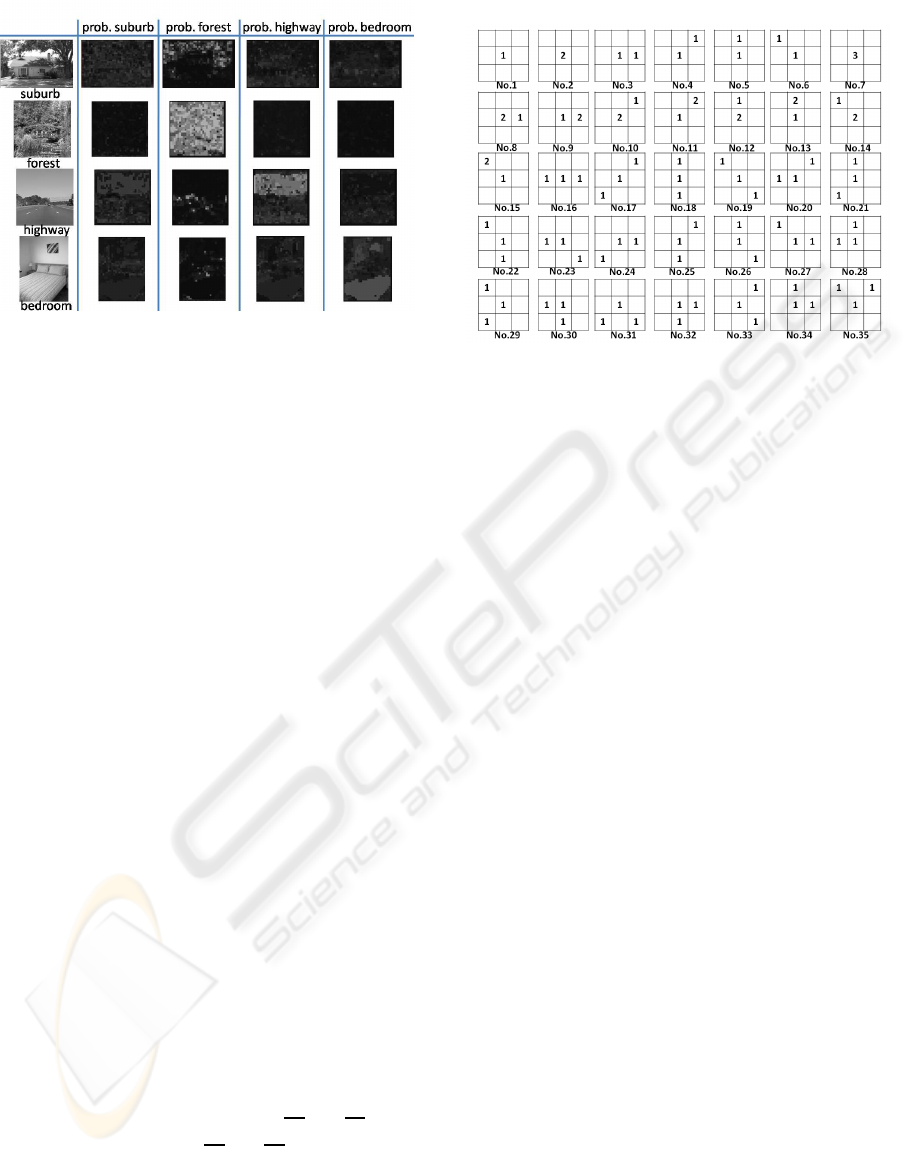
Figure 2: Posterior probability images.
3.2 PHLAC
Autocorrelationis defined as the productof signal val-
ues from different points and represents the strong
co-occurrence of these points. HLAC (Otsu and Ku-
rita, 1988) has proposed for extracting spatial auto-
correlations of intensity values. To capture the spa-
tial autocorrelations of posterior probabilities, the fea-
ture called PHLAC is designed by HLAC features of
posterior probability images. Namely, the Nth order
PHLAC is defined as follows.
R(c,a
1
,...,a
N
) =
Z
I
p
P(c|V
VQ(r)
)P(c|V
VQ(r+ a
1
)
)
· · ·P(c|V
VQ(r + a
N
)
)dr. (2)
In practice, many forms of Eq. (2) can be obtained by
varying the parameters N and a
n
. These parameters
are restricted to the following subset: N ∈ {0,1, 2}
and a
nx
,a
ny
∈ {±∆r × p,0}. In this case, HLAC
feature can be calculated by sliding predetermined
mask patterns. By eliminating duplicates that arise
from shifts of center positions, the mask patterns of
PHLAC can be represented as shown in Figure 3.
Larger Mask Patterns. Larger mask patterns are ob-
tained by varying the spatial interval ∆r. By calcu-
lating the autocorrelations in local regions, PHLAC
becomes robust against small spatial difference and
noise. Namely, P(c|V
VQ(r+ a
n
)
) in E.q.(2) is re-
placed to the local averaged posterior probability
L
a
(P(c|V
VQ(r+ a
n
)
)). Local averaging is calculated
in the rectangle region in which (x−
a
nx
2
,y−
a
ny
2
) is the
upper left corner, and (x+
a
nx
2
,y+
a
ny
2
) is the lower left
corner. The example of a larger mask pattern is shown
in Figure 4.
In previous paper, PHLAC feature was calculated
by using a single spatial interval. Recently, HLAC
feature was extended to 8th order and the multi-scale
Figure 3: Mask pattern for PHLAC. No.1 is 0th order, No.2-
6 are 1st order, and No.7-35 are 2nd order. The numbers
{1,2,3} of the mask patterns show the frequency at which
their pixel value is used for obtaining the product expressed
in Eq. (2).
spatial interval(Toyoda and Hasegawa, 2007). It was
not obvious that how many order of autocorrelations
and the multi-scale spatial interval are effective for
PHLAC. We confirmed that the multi-scale spatial
interval is effective for scene classification, and the
order of autocorrelation is sufficient upto 2nd order.
Effectiveness of PHLAC. PHLAC is an extension of
the bag-of-features approach. It was shown that 0th
order PHLAC has the almost same property of bag-
of-features, when linear classifiers are used. Addi-
tionally, higher order features of PHLAC have spa-
tial distribution informations of each posterior prob-
ability image. Therefore, PHLAC is possible to
achieve higher classification performances than bag-
of-features.
Furthermore, the desirable property of PHLAC is
its shift invariance. PHLAC uses spatial informations
by the meaning of relative positions of local regions
that are robust to spatial misalignment in shift than
histogram in spatial grids. Thus, the integration by
spatial autocorrelations could be better approach to
integrate the local posterior probabilities.
The autocorrelation of PHLAC is calculated on
each posterior probability image of category. Thus,
the dimension of PHLAC is (# of mask patterns ×
C) × # of spatial intervals. However, the crosscorre-
lation between other categories could contains more
richer informations for classification.
SCENE CLASSIFICATION USING SPATIAL RELATIONSHIP BETWEEN LOCAL POSTERIOR PROBABILITIES
327
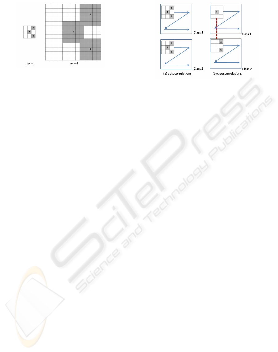
Figure 4: Larger mask pattern. Autocorrelation of larger re-
gions is realized by varying the parameter of spatial interval
∆r. The local averaged areas are indicated in gray area.
4 SPATIAL RELATIONSHIP
BETWEEN LOCAL
POSTERIOR PROBABILITIES
4.1 CIPHLAC
To capture more richer information between posterior
probability images, such as a road like region is left
to a forest like region, we extend the autocorrelation
of PHLAC to auto/crosscorrelations between poste-
rior probabilities of different categories. The differ-
ence between the autocorrelation and crosscorrelation
is shown in Figure 5. We call this method as cate-
gory index probability higher order autocorrelations
(CIPHLAC). The N-th order CIPHLAC is defined as
follows.
R(c
0
,..,c
N
a
1
,..,a
N
) =
Z
I
p
P(c
0
|V
VQ(r)
)P(c
1
|V
VQ(r + a
1
)
)
· · ·P(c
N
|V
VQ(r + a
N
)
)dr. (3)
Similar with the case of PHLAC, the parameters N
and a
n
are restricted to the following subset: N ∈
{0,1, 2} and a
nx
,a
ny
∈ {±∆r × p, 0}. Also, the
auto/crosscorrelations are calculated by regions and
the multi-scale spatial interval is used. To avoid the
increase of dimensions, we restrict the combination of
category index for 2nd order as follows: (c
0
, c
1
, c
2
) =
(c
0
, c
1
, c
1
). The calculation of CIPHLAC is realized
by extending PHLAC mask patterns(Figure 6). Note
that this mask pattern contains both autocorrelations
and crosscorrelations. The dimension of CIPHLAC
becomes ( C + # of 1st and 2nd order mask patterns
× C
2
)× # of spatial intervals.
Figure 5: Comparison of autocorrelations and crosscorrela-
tions. (a) autocorrelation calculates correlation among pos-
terior probabilities of each category. (b) crosscorrelaiton
calculates correlation among posterior probabilities of dif-
ferent categories.
4.2 CIPLAS
CIPHLAC uses only the products between local pos-
terior probabilitiesof differentcategories. Another re-
lationship operation may capture another feature be-
tween posterior probability images. Here, we propose
a subtraction operation of posterior probabilities. In
this paper, only 1st order subtraction is considered.
We define this method as category index probabil-
ity local autosubtraction (CIPLAS). The method con-
struct the sum of subtraction values by distinguishing
the positive and negative values. Namely, the defini-
tion of CIPLAS is given as follows.
R
+
(c
0
,c
1
a
1
) =
Z
I
p
Ψ
+
P(c
0
|V
VQ(r)
) − P(c
1
|V
VQ(r+ a
1
)
)
dr,
Ψ
+
(x) =
0(if x ≤ 0),
x(if x > 0).
R
−
(c
0
,c
1
a
1
) =
Z
I
p
Ψ
−
P
c
0
|V
VQ(r)
) − P(c
1
|V
VQ(r+ a
1
)
dr,
Ψ
−
(x) =
|x|(if x ≤ 0),
0(if x > 0).
(4)
Similar with the case of PHLAC, the parame-
ters N and a
n
are restricted to the following sub-
set: N ∈ {0,1, 2} and a
nx
,a
ny
∈ {±∆r × p,0}.
Also, the auto/crosssubtractions are calculated by re-
gions, and the multi-scale spatial interval is used.
In this paper, we use the 1st order mask patterns
(No.2-6) in PHLAC mask patterns. Thus, the di-
mension of CIPLAS is (2× number of 1st order
mask patterns × C
2
)×# of spatial intervals. Be-
cause auto/crosscorrelation values becomes high if
VISAPP 2010 - International Conference on Computer Vision Theory and Applications
328
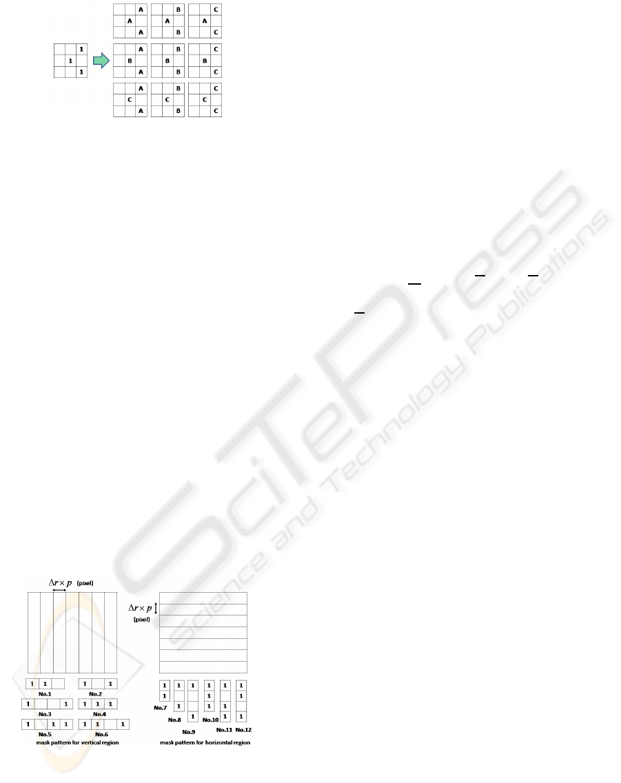
Figure 6: Mask patterns for CIPHLAC that restricted center
and the other category index. (A, B, C) shows a category
index.
the two reference posterior probabilities are high, and
auto/crosssubtractionvalues becomeshigh if these are
different, CIPLAS may be used with CIPHLAC com-
plementary.
4.3 Vertical/Horizontal Mask Patterns
The original mask patterns for PHLAC calculate au-
tocorrelation of square block regions. In scene clas-
sification, it is also effective the relationship of ver-
tical or horizontal regions by neglecting y or x axis
information of the images. In this paper, we con-
sider auto/crosscorrelations of vertical and horizontal
regions as shown in Figure 7. Each posterior prob-
ability is averaged as in the upper of Figure 7 and
auto/crosscorrelations are calculated each local aver-
aged regions by sliding mask pattern described in the
bottom of Figure 7. These mask patterns can be used
for PHLAC, CIPHLAC, and CIPLAS. In the case of
CIPLAS, No.1, 2, 3, 7, 8, 9 of the mask patterns are
used, since CIPLAS is 1st order. Thus, the number
of the additional mask patterns is only 6. However,
these mask patterns were significantly effective for
CIPLAS.
Figure 7: Vertical and horizontal mask patterns.
4.4 Feature Compression using 2DPCA
Because the dimensions of 2nd order CIPHLAC and
CIPLAS are large, we compress the features vec-
tors. The most standard technique for dimension
compression is principal component analysis(PCA).
However, in the high dimensional and small sam-
ple data, the accurate covariance matrix for PCA can
not be calculated. For two-dimensional data com-
pression, two-dimensional principal component anal-
ysis(2DPCA)(Yang et al., 2004) has been proposed
to slove this problem. Because the CIPHLAC and
CIPLAS is viewed as two-dimensional data (combi-
nation of category index × mask patterns), so we
compress the feature vector by 2DPCA.
Let A denotes an m × n feature vector, and X de-
notes an n-dimensional unitary column vector. Here,
m is # of combinations of category index, and n is # of
mask patterns × # of spatial intervals. In 2DPCA, the
covariance matrix of PCA is replaced to the following
image covariance matrix G
t
,
G
t
=
1
M
J
∑
j=1
(A
j
− A)
t
(A
j
− A), (5)
where A is the average of all training samples A
j
,
(j=1,2,...J). The optimal projection vectors, X
1
,...,X
d
are obtained as the orthonormal eigenvectors of G
t
corresponding to the first d largest eigenvalues. The
projected feature vectors, Y
1
,...,Y
d
, are obtained by
using the optimal projection vectors, X
1
,...,X
d
as fol-
lowing equations.
Y
k
= AX
k
,k = 1,2,...,d. (6)
The obtained principal component vectors are used to
form an m × d matrix B = [Y
1
,· · ·,Y
d
]. We apply
second 2DPCA to B
t
for reduction both redundancy
of combination of category index and mask patterns.
Both 1st and 2nd order vectors are compressed by
2DPCA simultaneously and the compressed vectors
are concatenated to 0th order vectors.
5 EXPERIMENT
We performed experiments on Scene-15 dataset
(Lazebnik et al., 2006). The Scene-15 dataset con-
sists of 4485 images spread over 15 categories. The
fifteen categories contain 200 to 400 images each and
range from natural scene like mountains and forest to
man-made environments like kitchens and office. We
selected 100 random images per categories as a train-
ing set and the remaining images as the test set. Some
examples of dataset images are shown in Figure 8.
To obtain reliable results, we repeated the exper-
iments 10 times. Ten random subsets were selected
from the data to create 10 pairs of training and
test data. For each of these pairs a codebook was
created by using k-means clustering on training
SCENE CLASSIFICATION USING SPATIAL RELATIONSHIP BETWEEN LOCAL POSTERIOR PROBABILITIES
329
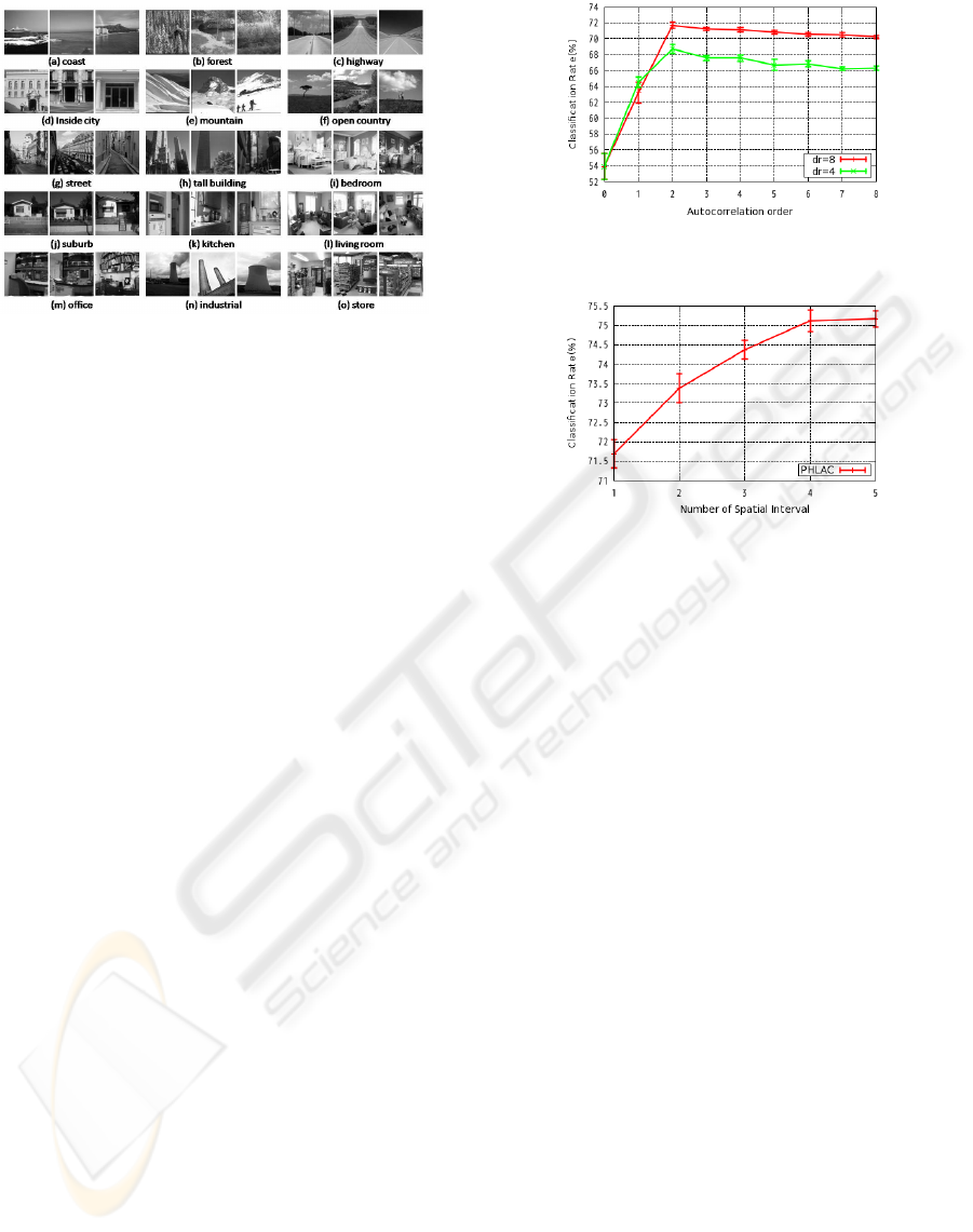
Figure 8: Example of Scene-15 dataset. Eight of these (a-
h) were originally collected in (Oliva and Torralba, 2001),
five (i-m) in (FeiFei and Perona, 2005), and two (n-o) in
(Lazebnik et al., 2006).
set. For classification, a linear SVM was used
by one-against-all. As implementation of SVM,
we used LIBLINEAR(Fan et al., 2008). Five-fold
cross-validation on the training set was carried out to
tune parameters of SVM. The classification rate we
report is the average of the per-class recognition rates
which in turn are averaged over the 10 random test
sets. As local features, we used a gradient local auto-
correlation(CLAC) descriptor (Kobayashi and Otsu,
2008) sampled on a regular grid. Because GLAC
can extract richer information than SIFT descriptor
and produce better performance. GLAC descriptor
used in this paper is 256-dimensional co-occurrence
histogram of gradient direction that contains 4 types
of local autocorrelation patterns. We calculated the
feature values from a 16×16 pixel patch sampled
every 8 pixels (i.e. p = 8), and histogram of each
autocorrelation pattern is L2-Hys normalized. In
the codebook creation process, all features sampled
every 24 pixel on all training images were used for
k-means clustering. The codebook size k is set to
400. As normalization method, we used L2-norm
normalization per autocorrelation order for PHLAC,
CIPHLAC, and CIPLAS. When using dimensional
compression, 2DPCA is applied after this nor-
malization and the compressed feature vector were
L2-norm normalizedusing all compressed dimension.
Autocorrelation-order. First, we compare the auto-
correlation order of PHLAC. The autocorrelation or-
der is changed from 0th to 8th order by using mask
patterns described in (Toyoda and Hasegawa, 2007).
The numbers of mask patterns for 3rd - 8th order
PHLAC are {153, 215, 269, 297, 305, 306} respec-
tively. In this comparison, single spatial interval ∆r ∈
{4,8} is used and feature vectors are not compressed.
The result is shown in Figure 9. The recognition rates
Figure 9: Recognition rates of PHLAC per number of auto-
correlation order.
Figure 10: Recognition rates of PHLAC per number of spa-
tial interval.
becomes better as to increase the autocorrelation or-
der upto 2nd. Therefore, the practical restriction of
autocorrelation order N ∈{0, 1, 2} was reasonable.
Number of Spatial Interval. Next, the number of
spatial interval is changed in 2nd order PHLAC. The
spatial interval is selected in the best combination
of ∆r ∈ {1, 2,4,8,12} by the first spilt classification
rates. In this comparison, feature vectors are not com-
pressed. The recognition rates per number of spatial
interval are shown in Figure 10. It can be confirmed
that the recognition rates becomes increase as to in-
crease the number of spatial interval.
Effectiveness of Relationship Between Posterior
Probability Images. The comparison between
PHLAC, CIPHLAC and CIPLAS is shown in Table
1. In this comparison, spatial interval ∆r = 8 is used
and feature vectors are not compressed. It is shown
that crosscorrelations between posterior probability
images improved classification performance of
PHLAC. For 1st order, the CIPHLAC had 8.89 %
better classification performance than PHLAC and
1.19 % for 2nd order. The recognition rates of
CIPLAS were also better than PHLAC for 1st order.
The combination of CIPHLAC and CIPLAS slightly
improved the recognition rates of CIPHLAC.
Effectiveness of Vertical/horizontal Mask Patterns.
The effectiveness of vertical/horizontal mask pat-
VISAPP 2010 - International Conference on Computer Vision Theory and Applications
330
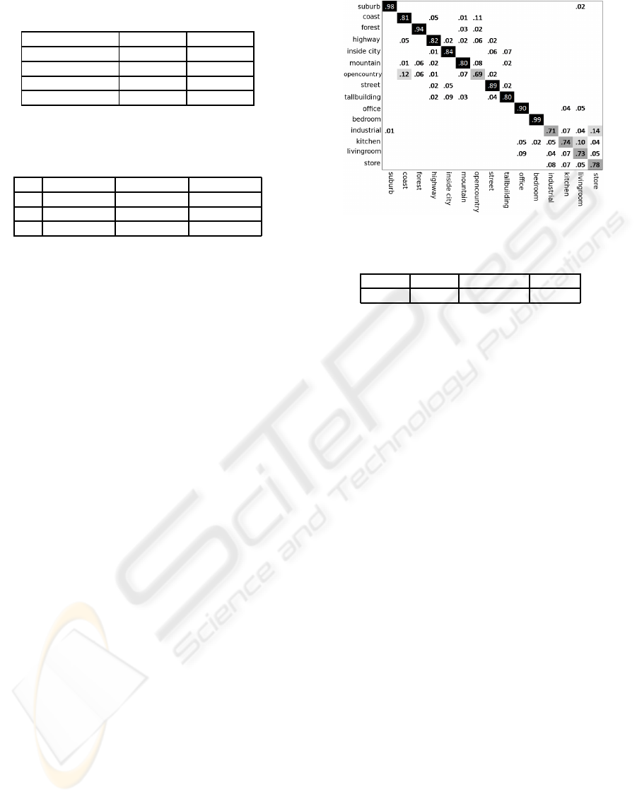
Table 1: Recognition rates of different relevant operations
(single spatial interval).
features 1st order 2nd order
PHLAC 63.19(± 1.29) 71.69(± 0.37)
CIPHLAC 72.08(± 0.51) 73.67(± 0.24)
CIPLAS 70.83(± 0.63) -
CIPHLAC + CIPLAS 72.45(± 0.60) 74.26(± 0.24)
Table 2: Recognition rates of vertical/horizontal mask pat-
terns. (a) standard mask patterns. (b) vertical/horizontal
mask patterns. (c) combination of (a) and (b).
PHLAC CIPHLAC CIPLAS
(a) 71.69(± 0.37) 73.67(± 0.24) 70.83(± 0.63)
(b) 71.77(± 0.30) 74.57(± 0.29) 76.46(± 0.23)
(c) 74.23(± 0.20) 75.61(± 0.21) 76.83(± 0.32)
terns are confirmed. In this comparison, spatial
interval ∆r = 8 is used and feature vectors are not
compressed. The experimental results are shown
in Table 2. By using only vertical/horizontal mask
patterns, the recognition rates of all methods out-
performed the original mask patterns. By using
both vertical/horizontal mask patterns and original
mask patterns, the recognition rates were improved.
The CIPLAS with vertical/horizontal mask patterns
exhibited the best performance.
Comparison with State of the Art. We used five
scales of spatial interval ∆r = (1, 2,4,8, 12) for both
original and vertical/horizontal mask patterns. We
compressed feature vectors by 2DPCA. We applied
2DPCA to the standard mask patterns and verti-
cal/horizontal(VH) mask patterns separability, and
concatenated these compressed vectors. The rank of
2DPCA is experimentally set using first spilt data.
The ranks (rank of category index combination, rank
of mask pattern) used in this experiment for each
method are: (50, 80) for CIPHLAC, (50, 40) for CI-
PHLAC(VH mask patterns), (60, 40) for CIPLAS,
(80, 20) for CIPLAS(VH mask patterns). The clas-
sification results of our proposed methods are shown
in upper of Table 4. CIPLAS with vertical/horizontal
mask patterns exhibited the best performance in pro-
posed methods. The confusion matrix of CIPLAS
with vertical/horizontal mask patterns is shown in
Figure 11. For the baseline of our proposed meth-
ods, we evaluated the two spatial gridded features by
using the same feature and codebook to ours. These
are:
(a) SPM(linear): the histogram of visual codebook
was created in the spatial pyramid grids as in the spa-
tial pyramid matching (Lazebnik et al., 2006).
(b) SP-PHLAC(0th): the 0th order PHLAC (i.e. sum
of posterior probabilities) was created in the spatial
pyramid grids as in the spatial pyramid matching.
Figure 11: Confusion matrix of CIPLAS with VH.
Table 3: Average required time per image (msec).
BOF PHLAC CIPHLAC CIPLAS
241.427 325.613 861.7 408.373
These method was classified by linear SVM to com-
pare the goodness of feature representations. The re-
sults of baseline methods are shown in the middle
of Table 4. Our methods significantly outperformed
these baseline methods. The comparison with the
state-of-the-art methods in Scene-15 dataset is shown
in the bottom of Table 4. Our method has the bet-
ter classification performance than spatial pyramid
matching (Lazebnik et al., 2006) without using spa-
tial grid informations and kernel methods. Further-
more, our method exhibited the best performance in
the method that uses linear classifiers.
Computational Cost. Table 3 shows the average
computation time of Scene-15 dataset in the feature
calculation process. One core of the quad core CPU
(Xeon 2.66 GHz), and C++ implementation were
used. In table 3, PHLAC, CIPHLAC, and CIPLAS
were calculated in 5 spatial intervals, and BOF is
the standard bag-of-features without spatial griding.
Since PHLAC is an extension of bag-of-features,
the method requires more computational costs than
bag-of-features. However, the method enables us to
achieve high accuracies with linear classifiers that can
calculate much faster than kernel methods. Although
CIPHLAC requires larger computational times than
PHLAC because the number of mask patterns is large,
CIPHLAC produces better accuracies than PHLAC.
6 CONCLUSIONS
We have proposed scene classification methods us-
ing spatial relationship between local posterior prob-
abilities. The autocorrelations of PHLAC feature are
SCENE CLASSIFICATION USING SPATIAL RELATIONSHIP BETWEEN LOCAL POSTERIOR PROBABILITIES
331

Table 4: Comparison with previous methods.
algorithm spatial classifier recognition rate
CIPHLAC(without VH) relative linear 80.37(± 0.37)
CIPLAS(without VH) relative linear 77.46(± 0.33)
CIPHLAC(with VH) relative linear 80.65(± 0.57)
CIPLAS(with VH) relative linear 82.63(± 0.25)
ALL relative linear 81.64(± 0.53)
SPM(linear)(Baseline) grid linear 72.60(± 0.27)
SP-PHLAC(0th)(Basel.) grid linear 68.29(± 0.22)
(Bosch et al., 2008) grid kernel 83.7
(Wu and Rehg, 2008) grid kernel 83.3(± 0.5)
(Lazebnik et al., 2006) grid kernel 81.4(± 0.5)
(Yang et al., 2009) grid linear 80.28(± 0.93)
(Zheng et al., 2009) grid kernel 74.0
extended to auto/crosscorrelations between posterior
probability images. The autosubtraction operator for
describing another spatial relationship between poste-
rior probability images, and vertical/horizontal mask
patterns for spatial layout of auto/crosscorrelations
are also proposed. Since the combination of cate-
gory index is large, the features are compressed by
2DPCA. Experiments using Scene-15 dataset have
demonstrated that the crosscorrelations between pos-
terior probabilities improves classification perfor-
mances of PHLAC, and auto/crosssubtraction with
vertical/horizontal mask patterns indicated the best
performance in our methods. The classification per-
formances of our methods in Scene-15 dataset were
competitive to the recent proposed methods without
using spatial grid informations and even using linear
classifiers.
REFERENCES
Battiato, S., Farinella, G., Gallo, G., and Ravi, D. (2009).
Spatial hierarchy of textons distributions for scene
classification. In MMM, pages 333–343.
Bosch, A., Munoz, X., and Freixenet, J. (2007). Segmenta-
tion and description of natural outdoor scenes. Image
and Vision Computing, 25:727–740.
Bosch, A., Zisserman, A., and Munoz, X. (2008). Scene
classification using a hybrid generative/discriminative
approach. IEEE Trans. on PAMI, 30(4):712–727.
Fan, R.-E., Chang, K.-W., Hsieh, C.-J., Wang, X.-R., and
Lin, C.-J. (2008). Liblinear: A library for large linear
classification. JMLR, 9:1871–1874.
Farinella, G., Battiato, S., Gallo, G., and Cipolla, R. (2008).
Natural versus artificial scene classification by order-
ing discrete fourier power spectra. In SSPR&SPR.
FeiFei, L. and Perona, P. (2005). A bayesian hierarchical
model for learning natural scene categories. In CVPR.
Gorkani, M. and Picard, R. (1994). Texture orientation for
sorting phots at a glance. In ICPR.
Hotta, K. (2009). Scene classification based on local auto-
correlation of similarities with subspaces. In ICIP.
Kobayashi, T. and Otsu, N. (2008). Image feature extraction
using gradient local auto-correlations. In ECCV.
Ladret, P. and Gue’rin-Dugue’, A. (2001). Categorisation
and retrieval of scene photographs from a jpeg com-
pressed database. Pattern Analysis & Applications,
4:185 – 199.
Lazebnik, S., Schmid, C., and Ponece, J. (2006). Beyond
bags of features: Spatial pyramid matching for recog-
nizing natural scene categories. In CVPR.
Matsukawa, T. and Kurita, T. (2009). Image classification
using probability higher-order local auto-correlations.
In ACCV.
Oliva, A. and Torralba, A. (2001). Modeling the shape of
the scene: A holistic representation of the spatial en-
velope. IJCV, 42(3):145–175.
Otsu, N. and Kurita, T. (1988). A new scheme for prac-
tical flexible and intelligent vision systems. In IAPR
Workshop on Computer Vision, pages 431–435.
Quattoni, A. and Torralba, A. (2009). Recognizing indoor
scenes. In CVPR, pages 413–420.
Rasiwasia, N. and Vasconcelos, N. (2008). Scene classifica-
tion with low-dimensional semantic spaces and weak
supervision. In CVPR, pages 1 – 8.
Renninger, L. and Malik, J. (2004). When is scene iden-
tification just texture recognition? Vision Research,
44(19):2301–2311.
Shotton, J., Johnson, M., and Cipolla, R. (2008). Semantic
texton forests for image categorization and segmenta-
tion. In CVPR, pages 1 – 8.
Szummer, M. and Picard, R. (1998). Indoor-outdoor im-
age classification. In IEEE Intl. Workshop on Content-
Based Access of Image and Video Databases.
Torralba, A. (2003). Contextual priming for object detec-
tion. IJCV, 53:169 – 191.
Torralba, A. and Oliva, A. (2003). Statistics of natural im-
age categories. Network: Computing in Nueral Sys-
tems, 14:391 – 412.
Toyoda, T. and Hasegawa, O. (2007). Extension of higher
order local autocorrelation features. Pattern Recogni-
tion, 40:1466–1477.
Vogel, J. and Schiele, B. (2007). Semantic modeling of nat-
ural scenes for content-based image retrieval. IJCV,
72(2):133–157.
Wu, J. and Rehg, J. (2008). Where am i: Place instance and
category recognition using spatial pact. In CVPR.
Yang, J., Yu, K., Gong, Y., and Huang, T. (2009). Linear
spatial pyramid matching using sparse coding for im-
age classification. In CVPR.
Yang, J., Zhang, D., Frangi, A., and Yang, J. (2004). Two-
dimensional pca: a new approach to appearance-based
face representation and recognition. IEEE Trans. on
PAMI, 26(1):131–137.
Yao, B., Niebles, J., and Fei-Fei, L. (2009). Mining discrim-
inative adjectives and prepositions for natural scene
recognition. In The joint VCL-ViSU 2009 workshop.
Zheng, Y., Lu, H., Jin, C., and Xue, X. (2009). Incorporat-
ing spatial correlogram into bag-of-features model for
scene categorization. In ACCV.
Zheng, Y.-T., Zhao, M., Neo, S.-Y., Chua, T.-S., and Tian,
Q. (2008). Visual synset: towards a higher-level visual
representation. In CVPR, pages 1 – 8.
VISAPP 2010 - International Conference on Computer Vision Theory and Applications
332
