SHAPE FROM SHADINGS UNDER PERSPECTIVE PROJECTION

AND TURNTABLE MOTION

Miaomiao Liu and Kwan-Yee K. Wong

Department of Computer Science, The University of Hong Kong, Pokfulam, Hong Kong

Keywords:

Two-frame-theory, Shape recovery, Turntable motion.

Abstract:

Two-Frame-Theory is a recently proposed method for 3D shape recovery. It estimates shape by solving a ﬁrst

order quasi-linear partial differential equation through the method of characteristics. One major drawback of

this method is that it assumes an orthographic camera which limits its application. This paper re-examines the

basic idea of the Two-Frame-Theory under the assumption of a perspective camera, and derives a ﬁrst order

quasi-linear partial differential equation for shape recovery under turntable motion. Dynamic programming is

used here to provide the Dirichlet boundary condition. The proposed method is tested against synthetic and

real data. Experimental results show that perspective projection can be used in the framework of Two-Frame-

Theory, and competitive results can be achieved.

1 INTRODUCTION

Shape recovery is a classical problem in computer

vision. Many constructive methods have been pro-

posed in the literature. They can generally be classi-

ﬁed into two categories, namely multiple-view meth-

ods and single-view methods. Multiple-view meth-

ods such as structure from motion (Tomasi, 1992)

mainly rely on ﬁnding point correspondences in dif-

ferent views, whereas single-view methods such as

photometric stereo use shading information to recover

the model.

Multiple-view methods can be further divided into

point-based methods and silhouette-based methods.

Point-based methods are the oldest technique for 3D

reconstruction (Pollefeys et al., 2001). Once feature

points across different views are matched, the shape

of the object can be recovered. The major draw-

back of such methods is that they depend on ﬁnd-

ing point correspondences between views. This is

the well-known correspondence problem which itself

is a very tough task. Moreover, point-based meth-

ods do not work for featureless object. On the other

hand, silhouette-based methods are a good choice for

shape recovery of featureless object. Silhouettes are

a prominent feature in an image, and they can be ex-

tracted reliably even when no knowledge about the

surface is available. Silhouettes can provide rich in-

formation for both the shape and motion of an object

(Wong and Cipolla, 2001; Liang and Wong, 2005).

Nonetheless, only sparse 3D points or a very coarse

visual hull can be recovered if the number of images

used for reconstruction is comparatively small. Pho-

tometric stereo, which is a single-view method, uses

images taken from one ﬁxed viewpoint under at least

three different illumination conditions. No image cor-

respondences are needed. If the albedo of the ob-

ject and the lighting directions are known, the surface

orientations of the object can be determined and the

shape of the object can be recovered via integration

(Woodham, 1980). However, most of the photometric

stereo methods consider orthographicprojection. Few

works are related to perspective shape reconstruction

(Tankus and Kiryati, 2005). If the albedo of the ob-

ject is unknown, photometric stereo may not be feasi-

ble. Very few studies in the literature use both shading

and motion cues under a general framework. In (Jin

et al., 2008), the 3D reconstruction problem is formu-

lated by combining the lighting and motion cues in

a variational framework. No point correspondences

is needed in the algorithm. However, the method in

(Jin et al., 2008) is based on optimization and requires

piecewise constant albedo to guarantee convergence

to a local minimum. In (Zhang et al., 2003), Zhang

et al. uniﬁed multi-view stereo, photometric stereo

and structure from motion in one framework, and

achieved good reconstruction results. Their method

has a general setting of one ﬁxed light source and one

camera, but with the assumption of an orthographic

camera model.

Liu M. and K. Wong K. (2010).

SHAPE FROM SHADINGS UNDER PERSPECTIVE PROJECTION AND TURNTABLE MOTION.

In Proceedings of the International Conference on Computer Vision Theory and Applications, pages 28-35

DOI: 10.5220/0002821300280035

 SciTePress

Similar to (Jin et al., 2008) , the method in (Zhang

et al., 2003) also greatly depends on optimization. A

shape recovery method was proposed in (Moses and

Shimshoni, 2006) by utilizing the shading and mo-

tion information in a framework under a general set-

ting of perspective projection and large rotation an-

gle. Nonetheless, it requires that one point correspon-

dence should be known across the images and the ob-

ject should have an uniform albedo.

A Two-Frame-Theory was proposed in (Basri and

Frolova, 2008) which models the interaction of shape,

motion and lighting by a ﬁrst order quasi-linear par-

tial differential equation. Two images are needed to

derive the equation. If the camera and lighting are

fully calibrated, the shape can be recoveredby solving

the ﬁrst order quasi-linear partial differential equa-

tion with an appropriate Dirichlet boundary condition.

This method does not require point correspondences

across different views and the albedo of the object.

However, it also has some limitations. For instance,

it assumes an orthographic camera model which is a

restrictive model. Furthermore, as stated in the paper,

it is hard to use merely two orthographic images of an

object to recover the angle of out-of-plane rotations.

This paper addresses the problem of 3D shape re-

covery under a ﬁxed single light source and turntable

motion. A multiple-view method that exploits both

motion and shading cues will be developed. The fun-

damental theory of the Two-Frame-Theory will be re-

examined under the more realistic perspective camera

model. Turntable motion with small rotation angle is

considered in this paper. With this assumption, it is

easy to control the rotation angle compared to the set-

ting in (Basri and Frolova, 2008). A new quasi-linear

partial differential equation under turntable motion is

derived, and a new Direchlet boundary condition is

obtained using dynamic programming. Competitive

results are achieved for both synthetic and real data.

This paper is organized as follows: Section 2 de-

scribes the derivation of the ﬁrst order quasi-linear

partial differential equation. Section 3 describes how

to obtain the Dirichlet boundary condition. Section 4

shows the experimental results for synthetic and real

data. A brief conclusion is given in Section 5.

2 FIRST ORDER QUASI-LINEAR

PDE

Turntable motion is considered in this paper. Simi-

lar to the setting in (Basri and Frolova, 2008), two

images are used to derive the ﬁrst order quasi-linear

partial differential equation (PDE). Suppose that the

object rotates around the Y-axis by a small angle. Let

X = (X,Y,Z) denotes the 3D coordinates of a point

on the surface. The projection of X in the ﬁrst im-

age is deﬁned as λ

= P

X, where P

is the projec-

tion matrix,

X is the homogenous coordinates of X

and

is the homogenous coordinates of the image

point. Similarly, the projection of X after the rota-

tion is deﬁned as λ

= P

X, where P

is the pro-

jection matrix after the rotation. The ﬁrst image can

be represented by I(x

), where (x

) is the inho-

mogeneous coordinates of the image point. Similarly

the second image can be represented by J(x

). Let

the surface of the object be represented by Z(X,Y).

Suppose that the camera is set on the negative Z-

axis. The unit normal of the surface is denoted by

n(X,Y) =

,−1)

⊤

√

,where Z

∂Z

∂X

and Z

∂Z

∂Y

After rotating the object by a small angle θ around the

Y-axis, the normal of the surface point becomes

(X,Y) =





cosθ 0 sinθ

0 1 0

−sinθ 0 cosθ









−1









cosθ−sinθ

−Z

sinθ−cosθ





(1)

Directional light is considered in this paper and it is

expressed as a vector l = (l

)

⊤

. Since the object

is considered to have a lambertian surface, the inten-

sities of the surface point in the two images are given

I(x

) = ρl

⊤

n =

ρ(l

+ l

−l

)

+ Z

+ 1

, (2)

J(x

) = ρl

⊤

ρ((l

cosθ−l

sinθ)Z

+ l

−l

sinθ−l

cosθ))

+ Z

+ 1

. (3)

where ρ is the albedo for the current point. If θ is

very small, (3) can be approximated by

J(x

) ≈

ρ((l

−l

θ)Z

+ l

−l

θ−l

))

+ Z

+ 1

. (4)

The albedo and the normal term (denominator) can be

eliminated by subtracting (2) from (4), and dividing

the result by (2). This gives

+ l

−l

)(J(x

) −I(x

))

= (−l

θ−l

θ)I(x

(5)

Note that some points may become invisible after ro-

tation and that the correspondences between image

SHAPE FROM SHADINGS UNDER PERSPECTIVE PROJECTION AND TURNTABLE MOTION

points are unknown beforehand. If the object has a

smooth surface, the intensity of the 3D point in the

second image can be approximated by its intensity in

the ﬁrst image through the ﬁrst-order 2D Taylor series

expansion:

J(x

) ≈ J(x

) + J

)(x

−x

) + J

)(y

−y

(6)

Therefore,

J(x

) −I(x

) ≈ J(x

) −I(x

)(x

−x

) + J

)(y

−y

(7)

Substituting (7) into (5) gives

+ l

I(x

)θ)Z

+ l

= −l

θI(x

) (8)

where

= J(x

) −I(x

) + J

)(x

−x

)

)(y

−y

Note that x

, y

, x

, and y

are functions of X, Y, and

Z, and (8) can be written more succinctly as

a(X,Y,Z)Z

+ b(X,Y, Z)Z

= c(X,Y,Z) (9)

where

a(X,Y,Z) = l

+ l

I(x

)θ,

b(X,Y,Z) = l

c(X,Y,Z) = −l

θI(x

). (10)

(9) is a ﬁrst-order partial differential equation in

Z(X,Y). Furthermore, it is a qusi-linear partial differ-

ential equation since it is linear in the derivatives of

Z, and its coefﬁcients, namely a(X,Y,Z), b(X,Y,Z),

and c(X,Y,Z), depend on Z. Therefore, the shape of

the object can be recovered by solving this ﬁrst or-

der quasi-linear partial differential equation using the

method of characteristics. The characteristic curves

can be obtained by solving the following three ordi-

nary differential equations:

dX(s)

= a(X(s),Y(s),Z(s)),

dY(s)

= b(X(s),Y(s),Z(s)),

dZ(s)

= c(X(s),Y(s),Z(s)), (11)

where s is a parameter for the parameterization of

the characteristic curves. (Basri and Frolova, 2008)

has given a detailed explanation of how the method

of characteristics works. It is also noticed that the

quasi-linear partial differential equation should have

a unique solution. Otherwise, the recovered surface

may not be unique. In the literature of quasi-linear

partial differential equation, this is considered as the

initial problem for quasi-linear ﬁrst order equations.

A theorem in (Zachmanoglou and Thoe, 1987) can

guarantee that the solution is unique in the neighbor-

hood of the initial boundary curve. However, the size

of the neighborhood of the initial point is not con-

strained. It mainly depends on the differential equa-

tion and the initial curve. It is very important to ﬁnd

an appropriate Dirichlet boundary. In this paper, dy-

namic programming is used to derive the boundary

curve.

3 BOUNDARY CONDITION

Under perspective projection, the Dirichlet Boundary

condition cannot be obtained in the same way as in

(Basri and Frolova, 2008). As noted in (Basri and

Frolova, 2008), the intensities of the contour genera-

tor points are unaccessible. Visible points (X

′

)

nearest to the contour generator are a good choice for

boundary condition. If the normal n

′

of (X

′

)

is known, Z

and Z

can be derived according to

n(X,Y) =

,−1)

⊤

√

. Note that (9) also holds for

′

). Therefore, (X

′

) can be obtained by

solving (9) with known Z

and Z

values. The prob-

lem of obtaining (X

′

) becomes the problem of

how to obtain n

′

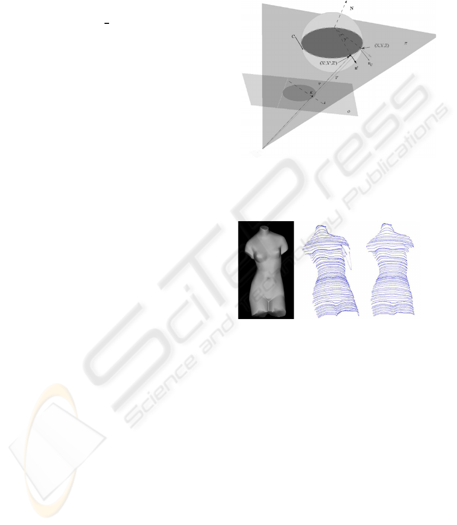
Let (X,Y,Z) be a point on the contour generator

(see Figure 1). Since (X,Y,Z) is a contour genera-

tor point, its normal n

must be orthogonal to its vi-

sual ray V. Consider a curve C given by the inter-

section of the object surface with the plane π deﬁned

by V and n

. In a close neighborhood of (X,Y,Z),

the angle between V and the surface normal along C

would change from just smaller than 90 degrees to

just greater than 90 degrees. Now consider a visible

point (X

′

) on C close to (X,Y,Z), its normal

′

should make an angle of just smaller than 90 de-

grees with V. If (X

′

) is very close to (X,Y, Z),

′

would also be very close to n

. To simplify the es-

timation of n

′

, it is assumed that n

′

is coplanar with

and lying on π. n

′

can therefore be obtained by

rotating n

around an axis given by the normal N of π

by an arbitrary angle γ. According to the lambertian

law, n

′

can be obtained by knowing the intensities of

corresponding points across different views and the

albedo. However, no prior knowledge of point cor-

VISAPP 2010 - International Conference on Computer Vision Theory and Applications

respondences and albedo ρ are available. Similar to

the solution in (Basri and Frolova, 2008), ρ and γ can

be obtained alternatively. The image coordinates of

the visible point nearest to the contour generator can

be obtained by searching along a line ℓ determined by

the intersection of the image plane o and π. As for

each γ in the range 0 < γ ≤

, a corresponding albedo

is computed and ρ is chosen as the mean of these

computed values. γ is then computed by minimizing

(I −ρl

⊤

R(γ)n

)

, where R(γ) is the rotation matrix

deﬁned by the rotation axis ℓ and rotation angle γ. n

′

is ﬁnally determined as R(γ)n

and (X

′

) can be

obtained by minimizing

bon

= ka(X

′

+ b(X

′

−c(X

′

(12)

Dynamic programming is used to obtain (X

′

Two more constraints are applied in the framework

of dynamic programming. One is called photometric

consistency which is deﬁned as

pho

(p) =

∑

(p) −l

⊤

(p))

, (13)

where p is a 3D point on the contour generator, and

(p) is a component of the normalized intensity mea-

surement vector which is composed of the measure-

ment of intensities in q neighboring views and n

(p)

is the normal of p in the q

neighboring view.

The other constraint is called surface smoothness

constraint which is deﬁned as:

con

(p, p

′

) = kpos(p) − pos(p

′

(14)

where pos(p) denotes the 3D coordinates of point p

and pos(p

′

) denotes the 3D coordinates of its neigh-

bor point p

′

along the boundary curve.

The ﬁnal Energy function is deﬁned as

E = µE

bon

+ ηE

pho

+ ωE

con

(15)

where µ, η, ω are weighting parameters. By mini-

mizing (15) for each visible point nearest to the con-

tour generator, the nearest visible boundary curve can

be obtained and used as Dirichlet Boundary condition

for solving (9).

4 EXPERIMENTS

The proposed method is tested on synthetic models

and real image sequence. The camera and light source

are ﬁxed and fully calibrated. Circular motion se-

quences are captured either through simulation or by

rotating the object on a turntable for all experiments.

Since the derivedﬁrst order quasi-linear partial differ-

ential equation is based on the assumption of small ro-

tation angle, the image sequences are taken at a spac-

ing of at most ﬁve degrees.

Figure 1: Computing boundary condition. The visible curve

nearest to contour generator is a good choice for the bound-

ary condition. The curve can be obtained by searching the

points whose normal is coplanar with those of the respective

contour generator points.

Figure 2: Shadow effect for shape recovery. Left column:

original image for one view used for shape recovery and

shadow appears near the left arm of the Venus model. Mid-

dle column: characteristic curves without using intensity

difference threshold for the solution of partial differential

equation. Right column: characteristic curves after using

intensity difference threshold for the solution of partial dif-

ferential equation.

It has been assumed that the synthetic model has a

pure lambertian surface since the algorithm is derived

according to the lambertian surface property. It is also

quite important to get good boundary conditions for

solving the partial differential equations.

As for synthetic experiment, it is easier to gen-

erate the image without specularities. However, it is

hard to control the image sequence without shadows

due to the lighting directions and the geometry of the

object. From (9), (10), and (11), it can be noted that

the solution of the ﬁrst order quasi-linear partial dif-

ferential equation mainly depends on the change of

the intensities in the two images. If the projection of

the point in the ﬁrst view is in shadow, the estima-

SHAPE FROM SHADINGS UNDER PERSPECTIVE PROJECTION AND TURNTABLE MOTION

Figure 3: Reconstruction of the synthetic sphere model with uniform albedo. The rotation angle is 5 degrees. Light direction

is [0, 0, −1]

⊤

, namely spot light. Camera is set on the negative Z-axis. Left column: two original images. Middle column:

characteristic curves for frontal view (top) and the characteristic curves observed in a different view (bottom). Right column:

reconstructed surface for front view (top) and the reconstructed surface in a different view (bottom).

Figure 4: Shape recovery for the synthetic cat model. Left column: two images used for reconstruction. Middle column:

characteristic curves for the view corresponding to the top image in the left column (top) and the characteristic curves observed

in a different view (bottom).Right column: Recovered shape with shadings in two different views.

tion of the image intensity using Taylor expansion in

the second view will also be inaccurate. The charac-

teristic curves will go crazy (see Figure 2). In order

to avoid the great error caused by shadow effect, the

intensity difference for the estimation points should

not be larger than a threshold δ

thre

which is obtained

through the experiments.

4.1 Experiment with Synthetic Model

The derived ﬁrst order quasi-linear partial differential

equation is applied to three models, namely the sphere

model, cat model, and Venus model. δ

thre

= 51 is used

for all the synthetic experiments to avoid the inﬂuence

of shadow in the image.

The ﬁrst simulation is implemented on the sphere

model. Since the image of the sphere with uniform

VISAPP 2010 - International Conference on Computer Vision Theory and Applications

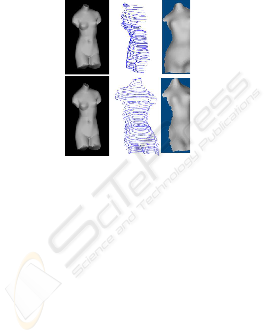
Figure 5: Shape recovery for the Venus model. Left column: two images used for shape recovery. Middle column: charac-

teristic curves for the view corresponding to the top image in the left column (top) and the characteristic curves observed in a

different view (bottom).Right column: Recovered shape with shadings in two different views.

albedo does not change its appearance after its ro-

tation around Y-axis (see Figure 3), only one image

is used to recover the 3D shape. Any small angle can

be used to the proposed equation. Nonetheless, if the

sphere has non-uniform albedo, two images will be

used for shape recovery. Figure 3 shows the original

images, the characteristic curves observed in two dif-

ferent views, and the recovered 3D shape examined

in two different views. The sphere model is assumed

to have a constant albedo. The reconstruction error is

tested by using k

Z −Zk

/kZk

, where

Z denotes the

estimated depth for each surface point and k·k

de-

notes the l

norm. The mean error is 4.63% for the

sphere with constant albedo which is competitive to

the result in (Basri and Frolova, 2008).

The second simulation is implemented on a cat

model. The image sequence is captured under gen-

eral lighting direction and with rotation angles at three

degrees spacing. Seven images are used to get the

boundary condition. Two neighboring images are

used for solving the derived quasi-linear partial dif-

ferential equation. The results are shown in Figure 4.

It can be observed that the body of the cat can be re-

covered except a few errors appeared at the edge. The

last simulation is implemented on a Venus model. The

sequence is taken at a spacing of ﬁve degrees.

Similarly seven images are used for getting the

boundary condition.

The front of the Venus model is recovered by us-

ing two neighboring view images for solving the de-

rived quasi-linear partial differential equation. The re-

sult is shown in Figure 5.

After the recovery of characteristics curves,

shapes for the Cat and Venus model with shadings are

shown by using the existing points to mesh software

VRmesh. The right columns of Figure 4, and Figure

5 show the results.

4.2 Experiment with Real Images

The real experimentis conducted on a ceramic mouse.

The mouse toy is put on a turntable. The relative po-

sitions of the lighting and the camera is ﬁxed. The

image sequence is taken by a Cannon 450D camera

with a 34 mm lens. The camera is calibrated using

a chessboard pattern and a mirror sphere is used to

calibrate the light. The image sequence is captured

with the rotation angle at ﬁve degree spacing. It can

be observed that there are specularities on the body of

the mouse. The intensity threshold is used to elimi-

nate the bad effect of the specularities since the pro-

posed algorithm only works well on lambertian sur-

SHAPE FROM SHADINGS UNDER PERSPECTIVE PROJECTION AND TURNTABLE MOTION

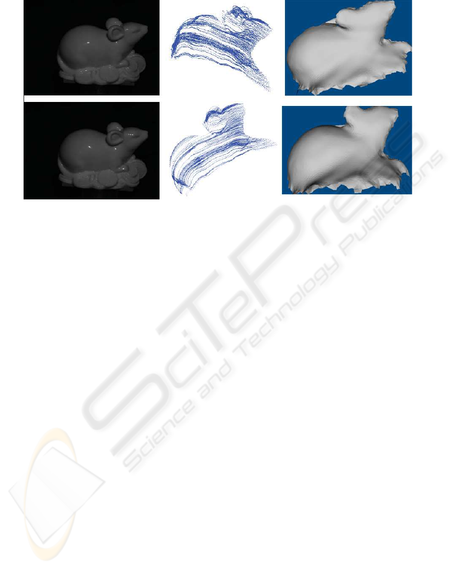
Figure 6: Shape recovery for a mouse toy. Left column: two images used for shape recovery. Middle column: characteristic

curves for the view corresponding to the top image in the left column (top) and the characteristic curves observed in a different

view (bottom).Right column: Recovered shape with shadings in two different views.

face. In order to avoid the shadow effect for solv-

ing the partial differential equation, δ

thre

= 27 is used

which is smaller than the value used in the synthetic

experiment since the captured images are compara-

tively darker. The original images and the charac-

teristic curves are shown in Figure 6. Although the

mouse toy has a complex topology and the images

have shadows and specularities, good results can be

obtained under this simple setting. Right column of

Figure 6 shows the results.

5 CONCLUSIONS

This paper re-examines the fundamental ideas of the

Two-Frame-Theory and derives a different form of

ﬁrst order quasi-linear partial differential equation for

turntable motion. It extends the Two-Frame-Theory

to perspective projection, and derives the Dirich-

let boundary condition using dynamic programming.

The shape of the object can be recovered by the

method of characteristics. Turntable motion is con-

sidered in the paper as it is the most common setup

for acquiring images around an object. Turntable mo-

tion also simpliﬁes the analysis and avoids the dif-

ﬁculty of obtaining the rotation angle in (Basri and

Frolova, 2008). The newly proposed partial differen-

tial equation makes the two frame method more use-

ful for a more general setting. Although the proposed

method is promising, it still has some limitations. For

instance, the proposed algorithm cannot deal with ob-

ject rotating with large angles. If the object rotates

with large angle, image intensities on the second im-

age cannot be approximated by the two dimensional

Taylor expansion. Some coarse-to-ﬁne strategies can

be used to derive new equations. In additions, the ob-

ject is assumed to have a lambertian surface and the

lighting is assumed to be a directional light source.

The recovered surface can be used as an initialization

for shape recovery method using optimization, which

can ﬁnally get a full 3D model. Further improvement

should be made before the method can be applied to

an object under general lightings and general motion.

REFERENCES

Basri, R. and Frolova, D. (2008). A two-frame theory of

motion, lighting and shape. In 2008 IEEE Computer

Society Conference on Computer Vision and Pattern

Recognition, 24-26 June 2008, Anchorage, Alaska,

USA, pages 1–7. IEEE Computer Society.

Jin, H., Cremers, D., Wang, D., Prados, E., Yezzi, A. J., and

Soatto, S. (2008). 3-d reconstruction of shaded objects

from multiple images under unknown illumination.

International Journal of Computer Vision, 76(3):245–

256.

Liang, C. and Wong, K.-Y. K. (2005). Complex 3d shape

recovery using a dual-space approach. In 2005 IEEE

Computer Society Conference on Computer Vision

and Pattern Recognition, 20-26 June 2005, San Diego,

CA, USA, pages 878–884.

Moses, Y. and Shimshoni, I. (2006). 3d shape recov-

ery of smooth surfaces: Dropping the ﬁxed view-

point assumption. In Computer Vision - ACCV 2006,

VISAPP 2010 - International Conference on Computer Vision Theory and Applications

7th Asian Conference on Computer Vision, Hyder-

abad, India, January 13-16, 2006, Proceedings, Part

I, volume 3851 of Lecture Notes in Computer Science,

pages 429–438. Springer.

Pollefeys, M., Vergauwen, M., Verbiest, F., Cornelis, K.,

and Gool, L. V. (Jun. 2001). From image sequences

to 3d models. In In Proceedings 3rd international

workshop on automatic extraction of man-made ob-

jects from aerial and space images, pages 403–410.

Tankus, A. and Kiryati, N. (2005). Photometric stereo

under perspective projection. In 10th IEEE Interna-

tional Conference on Computer Vision , 17-20 Octo-

ber 2005, Beijing, China, pages 611–616.

Tomasi, C. (1992). Shape and motion from image streams

under orthography: a factorization method. Interna-

tional Journal of Computer Vision, 9:137–154.

Wong, K.-Y. K. and Cipolla, R. (2001). Structure and mo-

tion from silhouettes. In 8th International Confer-

ence on Computer Vision,July 7-14, 2001, Vancouver,

British Columbia, Canada, pages 217–222.

Woodham, R. (Jan. 1980). Photometric method for deter-

mining surface orientation from multiple images. In

OptEng 19(1), pages 19(1):139–144.

Zachmanoglou, E. C. and Thoe, D. W. (1987). Introduc-

tion to partial differential equations with applications.

Dover Publications, New York:SUS.

Zhang, L., Curless, B., Hertzmann, A., and Seitz, S. M.

(2003). Shape and motion under varying illumina-

tion: Unifying structure from motion, photometric

stereo, and multi-view stereo. In 9th IEEE Interna-

tional Conference on Computer Vision, 14-17 October

2003, Nice, France, pages 618–625.

SHAPE FROM SHADINGS UNDER PERSPECTIVE PROJECTION AND TURNTABLE MOTION