
DISPARITY MAPS FOR FREE PATH DETECTION
Nuria Ortigosa
Centro de Investigaci
´
on en Tecnolog
´
ıas Gr
´
aficas, Universidad Polit
´
ecnica de Valencia
Camino de Vera s/n, 46022 Valencia, Spain
Samuel Morillas
Instituto de Matem
´
atica Pura y Aplicada, Universidad Polit
´
ecnica de Valencia
Camino de Vera s/n, 46022 Valencia, Spain
Guillermo Peris-Fajarn
´
es, Larisa Dunai
Centro de Investigaci
´
on en Tecnolog
´
ıas Gr
´
aficas, Universidad Polit
´
ecnica de Valencia
Camino de Vera s/n, 46022 Valencia, Spain
Keywords:
Computer vision, Stereo vision, Disparity maps, Assisted navigation.
Abstract:
In this paper we introduce a method to detect free paths in real-time using disparity maps from a pair of rectified
stereo images. Disparity maps are obtained by processing the disparities between left and right rectified images
from a stereo-vision system. The proposed algorithm is based on the fact that disparity values decrease linearly
from the bottom of the image to the top. By applying least-squares fitting over groups of image columns to a
linear model, free paths are detected. Only those pixels that fulfil the matching requirements are identified as
free path. Results from outdoor scenarios are also presented.
1 INTRODUCTION
Detecting free paths instead of detecting the obsta-
cles of the scene addresses a different and new point
of view regarding the aid for navigation without colli-
sions. Thus, there are a great number of references for
obstacle detection and not so many for free space de-
tection. Free path detection offers an advantage over
the obstacle detection: free pathways are easier to de-
tect looking at the pattern they follow in a disparity
map. Disparity decreases linearly from the bottom of
the image to the top, so free paths can be detected
faster with less computational cost looking for pixels
that match this pattern.
Among the reported works on obstacle-free space
detection we can find different approaches. For in-
stance, the method in (T. H. Nguyen and Nguyen,
2007) uses the Sum of Absolute Differences between
images meanwhile (E. Grosso, 1995) uses the time-to-
impact to objects in the scene to determine free-space.
To establish a path to guide a robot (M. Vergauwen,
2003) processes the disparity map and then provides
a measure for the cost of traversal (Travel Cost Map),
choosing the path which has the least associate cost.
(R. Labayrade, 2002) and (Y. Baudoin, 2009) detect
obstacles by means of the “v-disparity” image mean-
while (J.P. Tarel and Charbonnier, 2007) proposes a
direct approach for 3D road reconstruction. Occu-
pancy grids are used in (H. Badino and Franke, 2008)
and (H. Badino, 2007) for free space computation, de-
pending on the likelihood of each grid to be occupied
or not, meanwhile (U. Franke, 2000) applies a dis-
tance dependent threshold to depth maps obtained by
correlation between two stereo images and (A. Wedel
and Cremers, 2008) represents the ground plane as
a parametric B-spline surface. During last years,
obstacle-free space detection has been researched by
many authors, especially for intelligent automotive
and robotic applications, in order to aid automotive
navigation without collisions. Thus, in order to help
navigation, there are authors who detect and classify
obstacles (Y. Huang, 2005), detect the painted lane
markings (M. Bertozzi, 1998), find the optimum road-
obstacle boundary (S. Kubota, 2007), deduce the most
appropriate direction to avoid obstacles (L. Nalpan-
tidis and Gasteratos, 2009) or estimate diameters of
310
Ortigosa N., Morillas S., Peris-Fajarnés G. and Dunai L. (2010).
DISPARITY MAPS FOR FREE PATH DETECTION.
In Proceedings of the International Conference on Computer Vision Theory and Applications, pages 310-315
DOI: 10.5220/0002821603100315
Copyright
c
SciTePress

trees en the scene to determine whether or not they
are traversable obstacles (A. Huertas, 2005).
Most of the reported works use images from a
stereo-vision system, since the use of stereo cameras
allows the calculation of disparities for each pixel in
every frame, which is a key feature to perform an
accurate detection. The disparity of an image pixel
refers the location difference between the pixel in the
left image and the corresponding pixel in the right im-
age after both images have been rectified. Clearly, the
lower the disparity for a pixel is, the higher the dis-
tance up to the point represented by this pixel.
This paper presents an algorithm for the detection
of free paths in real-time, which is integrated in the
Cognitive Aid System for Blind and Partially Sighted
People (CASBliP) project (
http://www.casblip.
com
). The main aim of CASBliP is to develop a
system capable of interpreting and managing real
world information from different sources to support
mobility-assistance to any kind of visually impaired
users. This way, it assists the users to navigate their
way outdoors along pavements. There are also several
works whose aim is to help people in their naviga-
tion, by means of using GPS (J.M. Loomis, 1998), de-
tecting doorways (M. Snaith, 1998), crosswalks and
staircases (S. Se, 2003) or the obstacles in the scene
(N. Molton, 1998). The difference between CASBliP
Project and other references which also relay scene
information to the blind user (as (P.D. Picton, 2008))
lies in the portability of the system. In CASBliP, the
device works onboard the visually impaired person.
Thus, stereo cameras are constantly moving and the
scene often contains blurred and deformed objects.
The motivation of this work is the necessity of detect-
ing surrounding obstacle-free space in real-time to as-
sist in navigation applications. The proposed method
introduces the innovation of using disparity maps ob-
tained by the stereovision system to detect the sur-
rounding obstacle-free space by matching with a lin-
ear model.
The paper is organized as follows. The system
where the proposed algorithm is included and the
method to obtain disparity maps are described in Sec-
tion 2. The proposed method for free paths detection
is detailed in Section 3. Section 4 presents experi-
mental results and, finally, conclusions are drawn in
Section 5.
2 DISPARITY MAPS
The stereo-vision system comprises two Firewire
CCD stereo cameras providing 240 × 320 pixel im-
ages which are calibrated so that estimated internal
and external parameters are used to rectify the ac-
quired images. Correspondence between left and
right images takes place while minimizing a cost
function, followed by disparity and depth estimation.
In (D. Scharstein, 2002), existing stereo methods
are compared and their performance is evaluated with
different experiments with indoor images. Further-
more, they keep updated the state-of-the-art in a ta-
ble with the evaluation of up to 65 references of dif-
ferent authors (
http://vision.middlebury.edu/
stereo/
). Many of them, such as (Q. Yang, 2009)
and (C. Lawrence Zitnick, 2007) offer very accurate
disparity maps but can not be used for real-time ap-
plications, since they have runtime of seconds.
We have studied different algorithms for disparity
map estimation and we finally have chosen (S. Birch-
field, 1999) because this approach provides a good
trade-off between computational efficiency (about 8-
10 disparity maps per second) and quality of re-
sults. Moreover, it is based on dynamic programming,
which performs better than other approaches for out-
door scenes.
According to (S. Birchfield, 1999), disparity maps
are represented as N× M gray-scale images where the
gray level of each pixel is associated with its nearness,
as we can observe in Equation 1, where Z is the depth,
f is the focal length of the cameras, B is the baseline
of the stereo system and d is the disparity. Hence,
darker disparity map areas are associated to further
regions of the scene.
Z =
f ∗ B
d
(1)
The performance of the disparity map algorithm is
illustrated in Figure 1, where we show three examples
of stereovision images before being rectified and its
corresponding disparity maps computed.
We propose to determine free space areas by pro-
cessing only the 25% last rows of the disparity maps
(from row N − N/4 to row N), since these rows rep-
resent the scenario region that the user will first walk
through.
3 ALGORITHM DETAILS
The detection algorithm presented in this paper is
based on the fact that disparity map grey levels in
free space areas decrease slightly and linearly from
the bottom of the image to the top. On the other hand,
obstacles for which depth is approximately constant
are represented by flat zones. Figure 2 illustrates this
behaviour.
DISPARITY MAPS FOR FREE PATH DETECTION
311
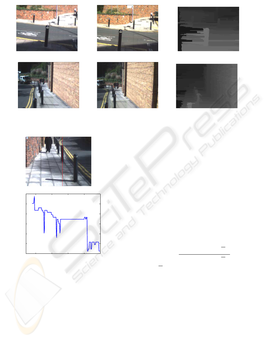
Figure 1: Examples of stereo images and depth maps. Left and right images are shown in first and second columns respectively
and third column shows the corresponding disparity maps computed using (S. Birchfield, 1999).
050100150200
20
40
60
80
100
120
140
Row number
Grey level
Figure 2: First row: Free path example and obstacle in left
image from the stereo system. Second row: grey levels of
the disparity map for the marked column in the image. For
free paths (rows from 130 on), grey levels decrease linearly
from the bottom to the top of the disparity map. The pole
(rows 60 to 130) is represented as a constant grey level.
Obstacle-free area after the pole (rows 0 to 40) has grey
level variations, but these do not match a linear model, since
in this case the disparity map is very noisy for that region.
Given a rectified left image I
L
and a rectified
right image I
R
from a stereo-vision system, the depth
computed using (S. Birchfield, 1999) for pixel in
(row,column) location (i, j) is denoted by D(i, j). In
order to save computation time and also to reduce the
influence of present noise, we process the disparity
maps by averaging groups of G pixel columns, where
we set G = 4 which is appropriate for our depth maps
of size 230× 290. Thus, we obtain the averaged col-
umn
e
D(i,k) from the values of columns D(i, j), j =
4k− 3, 4k − 2,. . .,4k where i = N,N − 1,...,N − N/4
and k = 1,2, ..., M/4. Then, a least-squares fitting
over
e
D(i,k) is done to find the best linear fitting to ad-
just the averaged column points. This model, which
provides an estimate for
e
D(i,k), is given by:
ˆ
D(i,k) = a
k
i+ b
k
(2)
where i is the row number in the processed column
of the depth map,
ˆ
D(i,k) is the estimated depth, a
k
is the gradient and b
k
is the y-intercept of the linear
model. Regarding the obtained fitting, its correlation
index is defined as
I(k) =
∑
N−N/4
i=N
(
ˆ
D(i,k) −
D)
2
∑
N−N/4
i=N
(
e
D(i,k) −
D)
2
, (3)
where
D denotes the mean of the values in
e
D(i,k).
I(k) measures the goodness of the fit for the group of
columns D(i, j), j = 4k − 3,4k − 2,. ..,4k. I(k) may
take values in [0,1], where 0 means no correlation and
1 indicates a perfect correlation. According to above,
we will determine as free path only those groups of
columns for which we obtain a good adjustment to
the linear model. This implies to require a mini-
mum value I(k) > I
T
for considering the candidate
group of columns D(i, j), j = 4k − 3, 4k − 2,..., 4k as
an obstacle-free path. Also, according to our linear
model, disparity map grey level in free paths should
be decreasing from the bottom of the column to the
top. So, we also require that the value of the gradi-
ent a
k
should be lower than a negative threshold a
T
.
Algorithm 1 details the proposed detection algorithm.
VISAPP 2010 - International Conference on Computer Vision Theory and Applications
312

Algorithm 1: Proposed free path detection algorithm.
The image is partitioned into disjoint groups of1
G columns;
foreach disjoint group of G columns in the2
image do
Compute the averaged column
e
D(i,k);3
Adjust the parameters of the linear model4
ˆ
D(i,k) by LMS (2);
Compute the value of I(k) (3);5
if I(k) > I
T
and a
k
< a
T
then6
D(i, j),i = N,N − 1,...,N − 4, j =7
4k− 3,4k − 2,..., 4k are marked as free
path;
else8
D(i, j),i = N,N − 1,...,N − 4, j =9
4k− 3,4k − 2,..., 4k are marked as an
obstacle;
end10
end11
0.8cm12
3.1 Computational Analysis
Regarding the fact that the method has to work in real-
time, an analysis of the computation cost has been
made. Table 1 shows the result of processing a N× M
pixels disparity map. In our case, for G = 4, N = 230
and M = 290, it is necessary to compute 66700 sums
and 54190 products.
Table 1: Number of required operations by processed dis-
parity map.
Sums Products
Columns average
N×M(G−1)
4G
N×M
4×G
Least Minimum Squares
9×N×M
4×G
5×N×M
2×G
Correlation index
N×M
G
N×M
2×G
Total
N×M(G+12)
4×G
13×N×M
4×G
The method has been implemented in C program-
ming language. Under an ACER 5612 at 1.73GHz it
spends less than 40ms for each processed depth map,
so it is suitable for real-time processes.
4 EXPERIMENTAL RESULTS
In order to measure the detection algorithm perfor-
mance in an objective way, it was necessary to manu-
ally prepare some groundtruth images, in which each
pixel was marked as free-space or occupied by some
object. This way, the detected areas can be compared
with the groundtruth images pixel by pixel in order
to obtain objective measurements for the detection in
terms of True Positives, True Negatives, False Posi-
tives and False Negatives. True Positives (TP) are de-
fined as the pixels which have been detected as free-
space and they really are. True Negatives (TN) are the
pixels correctly classified as occupied. False Positives
(FP) are defined as the pixels incorrectly classified as
free-space. False Negatives (FN) are the pixels which
really are free-space, but have been classified as occu-
pied.
Due to the application of this detection algorithm,
it is more important not to have False Positives than to
have False Negatives, in order to avoid collisions with
obstacles in the scene. Precision (5) is the proportion
of true results (True Positives) for all pixels detected.
Accuracy (6) is the proportion of correct detections
(both True Positives and True Negatives) in the tests.
Thus, we measure the performance of the method by
these parameters by defining a new statistic that we
name PACC given by
PACC =
Precision+ Accuracy
2
, (4)
where
Precision =
TP
TP+ FP
, (5)
Accuracy =
TP+ TN
TP+ TN + FP+ FN
(6)
4.1 Parameters Adjustment
A training set of 25 real outdoor training images and
their corresponding groundtruths have been used to
obtain appropriate settings for the algorithm detection
parameters. This set includes the most common sce-
narios that a person can run into outdoors (cars, free
paths, pedestrians, walls, poles...) in different illumi-
nating conditions (sunny and cloudy days, shadows of
surrounding objects...). This has been necessary since
the quality of disparity maps used for the detection
depends on the illumination conditions of the scene.
Disparity maps are less noisy when the scene is well
illuminated, since edges in the image are sharper and
it is easier to find the disparity between the left and
right images from the stereo-vision system.
It is very important to optimize the algorithm pa-
rameters in order to maximize the performance that
we measure in terms of PACC. Also, it is desirable to
have settings for the parameters that allow the method
to perform well for a variety of outdoor images. For
DISPARITY MAPS FOR FREE PATH DETECTION
313
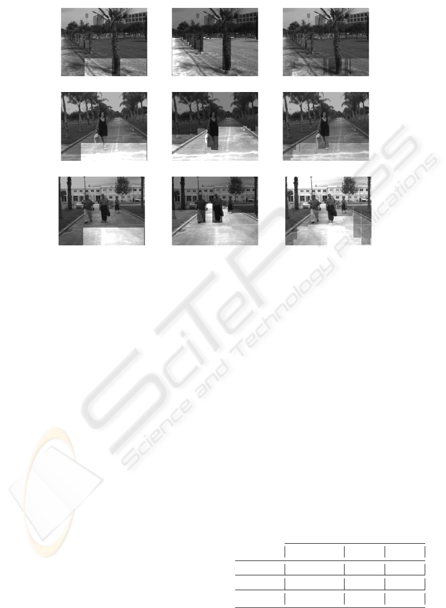
Figure 3: Examples of testing images. Brighter areas show detected free paths.First column shows results of the proposed
method, second column shows (S. Kubota, 2007) results and third column shows (H. Badino and Franke, 2008) results.
this reason, instead of obtaining the optimal values for
each image in the training set, we have found the sub-
optimal values of I
T
and a
T
that maximize the average
of PACC performance for the whole training set. The
parameters adjustment has been done in an iterative
way. Thus, once one parameter has been optimized it
is fixed, and we proceed to optimize the rest, repeat-
ing iteratively until convergence is reached.
We have varied I
T
from 0.2 to 0.99 and a
T
from -3
to 1, in steps of 0.01. We have obtained that I
T
= 0.4
and a
T
= −0.2 to be suboptimal for each image indi-
vidually, but the optimal values over all the training
set. Thus, we obtain about 84% of performance in
terms of PACC.
4.2 Algorithm Performance
In this section we assess the performance of the free
path detection method, using the previous suboptimal
settings for I
T
and a
T
.
We have compared the detection results of
our method with another two recent references
(H. Badino and Franke, 2008),(S. Kubota, 2007) for a
testing image set different from the training set used
for parameters adjustment. Figure 3 shows three dif-
ferent detection results examples for the three meth-
ods and Table 2 shows the Precision and Accuracy
values obtained for the whole testing set. These fig-
ures confirm that the algorithm works and detects free
paths properly.
The visual analysis reveals that sometimes some
free space areas are not detected. Usually, they cor-
respond to borders of the image or corners, untex-
tured areas (areas that can not be matched between
left and right stereoimages) or not well illuminated ar-
eas. However, we can see that in all cases we can de-
tect at least the wider free space area to walk through,
so the method performs appropriately for the purpose
of the project in which it is integrated.
Furthermore, as we have explained before, for our
application it is more important not to have False Pos-
itives than to have False Negatives in order to avoid
having collisions, although sometimes it leads to have
some False Negatives. Thus, maximizing True Posi-
tives means to maximize Precision. We can observe
that our method obtains similar values of Precision
compared with the other two references and it can be
used for real-time applications, owing to the fact of its
low computational cost.
Table 2: Performances for the testing image set.
Our method Kubota Badino
Precision 0.9926 0.9755 0.9981
Accuracy 0.7121 0.9744 0.8021
PACC 0.8523 0.9749 0.9001
VISAPP 2010 - International Conference on Computer Vision Theory and Applications
314

5 CONCLUSIONS AND FUTURE
WORK
In this paper we have presented a new method for free
path detection which is based on an analysis of dispar-
ity maps obtained from processing a pair of stereoim-
ages. The method is based on detecting as obstacle-
free areas the disparity map columns that match a lin-
ear model. For this, the best first-degree polynomial
adjusting the cloud of points is obtained by the least-
squares method and the obtained result is checked to
meet the desired requirements. Computational analy-
sis of the method has been done to assess its suitabil-
ity for real-time processing. An experimental study
has been used to derive suboptimal settings for the
method parameters. The method has been compared
with two of the most recent references in free space
detection and it provides good results. Future work
could focus on improving the algorithm performance
by including temporal coherence to track the detected
obstacle-free areas.
REFERENCES
A. Huertas, L. Matthies, A. R. (2005). Stereo-based tree
traversability analysis for autonomous off-road navi-
gation. In IEEE Computer Society. IEEE Workshop
on Applications of Computer Vision.
A. Wedel, U. Franke, H. B. and Cremers, D. (2008). B-
spline modeling of road surfaces for freespace estima-
tion. In IEEE. IEEE Intelligent Vehicles Symposium.
C. Lawrence Zitnick, S. B. K. (2007). Stereo for image-
based rendering using image over-segmentation. In-
ternational Journal of Computer Vision, 75(1):49–65.
D. Scharstein, R. S. (2002). A taxonomy and evalua-
tion of dense two-frame stereo correspondence algo-
rithms. International Journal of Computer Vision,
47(1/2/3):7–42.
E. Grosso, M. T. (1995). Active/dynamic stereo vision.
IEEE Transactions on Pattern Analysis and Machine
Intelligence, 17(9):868–879.
H. Badino, U. Franke, R. M. (2007). Free space com-
putation using stochastic occupancy grids and dy-
namic programming. Workshop on Dynamical Vision,
ICCV, Rio de Janeiro (Brazil).
H. Badino, R. Mester, T. V. and Franke, U. (2008). Stereo-
based free space computation in complex traffic sce-
narios. pages 189–192. IEEE Southwest Symposium
on Image Analysis & Interpretation.
J.M. Loomis, R.G. Golledge, R. K. (1998). Navigation sys-
tem for the blind: Auditory display modes and guid-
ance. Presence, 7(2):193–203.
J.P. Tarel, S. L. and Charbonnier, P. (2007). Accurate and
robust image alignment for road profile reconstruc-
tion. In IEEE. IEEE International Conference on Im-
age Processing.
L. Nalpantidis, I. K. and Gasteratos, A. (2009).
Stereovision-based algorithm for obstacle avoidance.
In Lecture Notes in Computer Science. Intelligent
Robotics and Applications.
M. Bertozzi, A. B. (1998). Gold: A parallel real-time stereo
vision system for generic obstacle and lane detection.
IEEE Transactions on Image Processing, 7(1):62–81.
M. Snaith, D. Lee, P. P. (1998). A low-cost system using
sparse vision for navigation in the urban environment.
Image and Vision Computing, 16(4):225–233.
M. Vergauwen, M. Pollefeys, L. V. G. (2003). A stereo-
vision system for support of planetary surface explo-
ration. Machine Vision and Applications, 14(1):5–14.
N. Molton, S. Se, J. B. e. a. (1998). A stereo vision-based
aid for the visually impaired. Image and Vision Com-
puting, 16(4):251–263.
P.D. Picton, M. C. (2008). Relaying scene information to
the blind via sound using cartoon depth maps. Image
and Vision Computing, 26(4):570–577.
Q. Yang, L. Wang, R. Y. e. a. (2009). Stereo match-
ing with color-weighted correlation, hierarchical be-
lief propagation, and occlusion handling. IEEE Trans-
actions on Pattern Analysis and Machine Intelligence,
31(3):492–504.
R. Labayrade, D. Aubert, J. T. (2002). Real time obstacle
detection in stereo vision on non-flat road geometry
through v-disparity representation. In INRIA. IEEE
Intelligent Vehicle Symposium.
S. Birchfield, C. T. (1999). Depth discontinuities by pixel-
to-pixel stereo. International Journal of Computer Vi-
sion, 17(3):269–293.
S. Kubota, T. Nakano, Y. O. (2007). A global optimization
for real-time on-board stereo obstacle detection sys-
tems. In IEEE. IEEE Intelligent Vehicles Symposium.
S. Se, M. B. (2003). Road feature detection and estimation.
Machine Vision and Applications, 14(3):157–165.
T. H. Nguyen, J.S. Nguyen, D. P. and Nguyen, H.
(2007). Real-time obstacle detection for an au-
tonomous wheelchair using stereoscopic cameras.
Conf Proc IEEE Eng. Med. Biol. Soc., 2007(1):4775–
4778.
U. Franke, A. J. (2000). Real-time stereo vision for urban
traffic scene understanding. In IEEE. IEEE Intelligent
Vehicles Symposium.
Y. Baudoin, D. Doroftei, G. D. C. e. a. (2009). View-finder:
Robotics assistance to fire-fighting services and crisis
management. In IEEE Computer Society. IEEE In-
ternational Workshop on Safety, Security, and Rescue
Robotics.
Y. Huang, S. Fu, C. T. (2005). Stereovision-based
object segmentation for automotive applications.
EURASIP Journal on Applied Signal Processing,
2005(14):2322–2329.
DISPARITY MAPS FOR FREE PATH DETECTION
315
