
A NOVEL PERFORMANCE METRIC FOR GREY-SCALE EDGE
DETECTION
Ian Williams
Faculty of Technology Engineering and the Environment, Birmingham City University, Birmingham B4 7XG, U.K.
David Svoboda
Faculty of Informatics, Masaryk university, Botanick´a 68a, 602 00 BRNO, Czech Republic
Nicholas Bowring
Department of Engineering and Technology, Manchester Metropolitan University, Manchester M1 5GD, U.K.
Keywords:
Edge detection, Grey-scale measure, Performance measure, Connectivity, Figure of merit.
Abstract:
This paper will discuss grey-scale edge detection evaluation techniques. It will introduce three of the most
common edge comparison methods and assess their suitability for grey-scale edge detection evaluation. This
suitability evaluation will include Pratt’s Figure Of Merit (FOM), Bowyer’s Closest Distance Metric (CDM),
and Prieto and Allen’s Pixel Correspondence Metric. The relative merits of each method will be discussed
alongside the inconsistencies inherent to each technique. Finally, a novel performance criterion for grey-scale
edge comparison, the Grey-scale Figure Of Merit (GFOM) will be introduced which overcomes some of the
evaluation faults discussed. Furthermore, a new technique for assessing the relative connectivity of detected
edges will be described and evaluated. Overall this will allow a robust and objective method of gauging edge
detector performance.
1 INTRODUCTION
Regardless of the technique used for edge detection;
Sobel, Prewitt (
ˇ
Sonka et al., 1986), Canny (Canny,
1986), or statistical, like the work of (Bowring et al.,
2004) and (Fesharaki and Hellestrand, 1994), the
evaluation will be the same and an effective perfor-
mance measure will be suitable for all.
Many evaluation methods are subjective in their
nature, usually conducted using the human percep-
tion of an edge, or with the aim of recognising any
objects contained within the image. This subjective
evaluation is an unsatisfactory performance test by it-
self, and overall objective measures like those of (Ab-
dou and Pratt, 1979), (Bowyer et al., 2001), (Boaven-
tura and Gonzaga, 2009) and (Prieto Segui and Allen,
2003), or a combination of both subjective and objec-
tive measures are more preferable as described in the
work of (Heath et al., 1996).
Objective performance determines the accuracy of
an edge detector, with restricted influence from hu-
man perception. However, although extensive study
has concentrated on the development and optimisa-
tion of edge detectors there has been little develop-
ment of an accurate measure to gauge their success.
The most common evaluation techniques asses per-
formance by comparing edges within the edge de-
tected image against a pre-segmented gold standard
image. This can be either user defined or automati-
cally computed as in the work of (Fern´andez-Garc´ıa
et al., 2008). However, many are gauged for binary
edge detection, or on images thresholded at an appro-
priate but subjective value as in the technique of (Ab-
dou and Pratt, 1979).This evaluation, while accurate
in its field, makes strong assumptions about the use-
fulness of the detected edges. Moreover, if taken out
of the application context for which it was designed,
or evaluated at a different threshold level, the signifi-
cance of any results can become questionable.
91
Williams I., Svoboda D. and Bowring N. (2010).
A NOVEL PERFORMANCE METRIC FOR GREY-SCALE EDGE DETECTION.
In Proceedings of the Inter national Conference on Computer Vision Theory and Applications, pages 91-97
DOI: 10.5220/0002821700910097
Copyright
c
SciTePress

2 EDGE DETECTION
PERFORMANCE
The three main criteria for edge detection were de-
fined by (Canny, 1986), namely the accurate detec-
tion of edges with the error rate to a minimum, the
accurate location of edges with regards to the ground
truth, and finally the single response to any edge en-
suring any multiple edge detection is avoided.
These three criteria form the basis of any edge
detection evaluation performance, which can be de-
scribed as:
True Positive: the sum of true edges detected,
False Positive: the sum of falsely detected edges,
True Negative: the sum of true non-edges detected
and False Negative: the sum of falsely detected non-
edges. In addition to this we can evaluate the “local-
isation”, which assesses the location accuracy of the
actual edge to the detected edge, and finally the “sin-
gle response” which evaluates if there is only a sin-
gle response to any one edge testing the possibility of
multiple responses to a single desired edge.
General correlation principles between the edge
detected image and the associated ground truth im-
age could be used to determine a simple performance
measure of the detector. For example a simple sub-
traction of the detected image and the ground truth
would determine the number of false positives and
false negatives. However such a simple evaluation
operation would not tolerate any shift in localisation
of true edges in the image. Subsequently, a detector
with even slight localisation errors would be unfairly
awarded a poor performance value. Evaluating with
reference to single pixel edges only would therefore
allow no tolerance for edges that were miss-aligned
by one pixel in the image. These problems were iden-
tified by (Grigorescu et al., 2003) who, through the
use of a pixel region mask, allowed for slight mis-
alignment errors and evaluated any non zero pixel
within this mask to be a true positive. As described
by in the work of (Joshi and Sivaswamy, 2006), this
method of performance is itself subjective and using
a larger mask will result in a greater number of false
positives being detected and therefore reduced perfor-
mance measure.
Although accurate for evaluating performance
against synthetic images, both true and false positive
or negative values should be approached with caution
when assessing performance of real images, or im-
ages with significant levels of texture. These mea-
sures can unduly bias a noisy background area of a
textured image and in the case on images where there
are only a few edges in relation to the background
area, can produce an inaccurately low performance
measure.
In addition to this problem, many evaluation mea-
sures are gauged for object oriented edge detection,
and therefore represent the result as a measure of ef-
fectiveness against final tasks, such as object recog-
nition. This evaluation, while accurate in its field,
makes strong assumptions about the usefulness of the
detected edges. Moreover, if taken out of the appli-
cation context, the significance of the results can be-
come questionable. To avoid this ambiguity the work
detailed in this paper performs an analysis of edge de-
tection in its entirety without determining a final ap-
plication step for the image. This allows evaluation
simply on the accuracy of the “true” edges within the
image and not just the object boundaries. This gives
a performance indicator that is useful for a variety of
post-edge detection applications.
To avoid any threshold ambiguity, and for appli-
cations which are reliant on the detection of accu-
rate grey-level edges, as in the work of (Svoboda and
Matula, 2003), a grey-scale evaluation should also be
used. Grey-scale assessment is not a simple task how-
ever, and work by (Prieto Segui and Allen, 2003) has
illustrated some of the difficulties. Their work evalu-
ated the noise robustness of several grey-scale evalu-
ation methods and highlighted inconsistencies inher-
ent to the CDM (Closest Distance Metric)(Bowyer
et al., 2001), PSNR (Peak Signal to Noise Ratio), and
the FOM (Figure of Merit) evaluation methods de-
signed by (Abdou and Pratt, 1979). To avoid these
problems (Prieto Segui and Allen, 2003) developed a
novel PCM (Pixel Correspondence Metric) technique,
which in practise was both sensitive and consistent in
its evaluation and gave more precision to the assess-
ment of edge quality.
3 PERFORMANCE METRICS
3.1 PCM (Pixel Correspondence
Metric)
The Pixel CorrespondenceMetric (or PCM) is the first
edge evaluation measure detailed in this work. PCM
evaluates all the pixel points in two given images
(PCM(a, b)), here represented as the edge detected
image (a) and the ideal ground truth image (b). For
each pixel point in the edge image a (a(i, j)) the met-
ric checks for an appropriate match within a defined
pixel neighbourhood in the ideal image b (b(i, j)).
Unlike comparison metrics which do not allow for a
shift in the detected pixel points, or simply evaluate
binary images, PCM evaluates the pixel match based
VISAPP 2010 - International Conference on Computer Vision Theory and Applications
92

on both the spatial distance between the pixel points
and also the actual grey-level value of the detected
edge point. Any non-matched pixel points are then
measured as errors. This error eliminates the pos-
sibility of multiple matches to the same edge point
through a process of weighted matching using bipar-
tite graphs. This form of bipartite matching ensures
that for every non-zero pixel point in the edge de-
tected image the PCM match value is maximised us-
ing the ideal, and therefore the overall PCM for the
match image is maximised. For the work presented
here the implementation of PCM by (Prieto Segui and
Allen, 2003) is used (See Equation 1). For a more de-
tailed explanation and the finer workings of this tech-
nique please refer to the work of (Prieto Segui and
Allen, 2003).
PCM
η
(a, b) = 100
1−
C(M
opt
(a, b))
|a
S
b|
(1)
where: C(M
opt
(a, b)) = the cost of optimal matching
between each image - calculated using weighted bi-
partite graphs
η = The maximum localisation error allowed between
pixels
|a
S
b| = The total number of non-zero pixels in image
a or b.
3.2 CDM (Closest Distance Metric)
The Closest Distance Metric (CDM) is an evaluation
technique based in the work of (Bowyer et al., 2001).
Similar in principle to the PCM metric, the CDM
technique uses a defined pixel region (η) to check
every pixel in the edge detected image array (a(i, j))
for a corresponding match in the ideal image (b(i, j))
across this region. The work by (Bowyer et al., 2001)
used binary edge images which allowed for the use
of Receiver Operating Characteristic (ROC) curves to
evaluate the trade off between true positive and false
positive rates. However in this work the relative per-
formance of grey-scale edge detection is assessed so
ROC curves would not be appropriate to use with the
CDM metric. This work uses the implementation of
CDM as defined by (Prieto Segui and Allen, 2003)
(see Equation 2). The implementation therefore al-
lows the comparison to be based on both the distance
and the grey-level strength of the actual edge against
the ideal edge.
CDM
η
(a, b) = 100
1−
C(M
c
d(a, b))
(|a
S
b|)
(2)
where: η = The size of the region for matching be-
tween images.
C(M
c
d(a, b)) = The cost of matching using a “closest-
distance” metric
|a
S
b| = The sum of non zero points in images a and
b.
3.3 PFOM (Pratt’s Figure of Merit)
The most commonly used form of edge comparison
measure was defined by (Pratt, 1978), and is regarded
as the standard in edge detection evaluation. The
Figure Of Merit (FOM) performance is assessed on
binary or threshold images against a pre-segmented
ground truth edited to include only their “true” edges.
Pratt’s Figure Of Merit (FOM) (Pratt, 1978) is defined
in Equation 3.
R =
1
I
sum
I
A
∑
i=1
1
1+ βd
2
i
(3)
where: I
sum
= max(I, I
A
). I = The sum of the ideal
edge points. I
A
= The sum of the detected edge points.
d
i
= the distance of the i
th
edge point from the ideal
edge point. β = A scaling constant (typically set to
1
9
).
The major drawbacks of the Pratt method of evalu-
ation is that it is designed to work with binary images
only. Therefore the implementation has been adapted
in this work for with grey-scale images.
3.4 GFOM (Grey-scale Figure of Merit)
It is often important to assess each image based on its
grey-levels before any threshold or post edge detec-
tion process has been applied, to accurately gauge the
effectiveness of each raw edge detector. This adapted
Grey-scale Figure Of Merit (or GFOM) that addresses
this requirement is now described.
The Figure Of Merit (FOM) performance is cal-
culated for each of the 256 grey levels in both the
edge detected and the ideal gold standard image inde-
pendently and is shown in Figure 1. This is achieved
by thresholding the image at each grey-scale level in
turn. A performance value can then be calculated for
that specific threshold level against the gold standard
image. The sum of these 256 performance values can
then be calculated, and the mean Figure of merit de-
termined by Equation 4. This can then be assigned as
the overall grey-scale performance value (GFOM) for
the image.
GFOM =
L
∑
i=1
R
i
L
(4)
A NOVEL PERFORMANCE METRIC FOR GREY-SCALE EDGE DETECTION
93

threshold
t=0edge image
gold standard
threshold
t=0
t=1
t=2
t=255
t=255
t=1
t=2
FOM FOM FOM FOM
Figure 1: GFOM is Pratts FOM adapted to work with 256
grey-scale levels. Both the edge image and ground-truth
image are threshold at each of the 256 grey-scale levels in
turn. Pratt’s Figure of merit is then calculated for the cur-
rent threshold level between both images. This process is
repeated for each of the 256 grey-scale levels and the sum
of Pratt merit Figures is calculated. The mean of these Pratt
values is then allocated as the Figure of merit for the image.
where:
L = the number of grey-scale levels (typically 256)
in both the edge detected image and the gold standard
image.
R
i
= the FOM value defined in Equation 3 with
threshold value “i = 1. . . L”.
3.5 Edge Connectivity
PCM, CDM, FOM and GFOM are not designed to as-
sess the “connectivity” of the edge. Consequently as
illustrated in the results section, an accurately located
edge which is fragmented or not continuous could be
awarded a greater performance metric than one which
is continuous but has slight localisation errors (See
Table 1 and Figures 4 d,e). To gauge the accuracy of
edge detectors the performance can be assessed as a
combination of both edge accuracy and edge connec-
tivity.
Here connectivity is defined as a function of the
total connected points along the “ridge” of the edge
without any sharp breaks. The overall connected edge
value for the assessed image can be defined as a func-
tion of the total non-zero pixels (i.e the detected edge
points) within the image. This technique is initially
based on the work of (Zhu, 1995). Unlike Zhu, who in
his work defines all the possible binary edge patterns
to assess edge connectivity, this work determines the
direction, and location of edges using a novel angle
finding technique, which is described in the next sec-
tion. Furthermore, this connectivity measure is again
for grey-level images so binary pixels patterns would
be of no use in this evaluation.
A
A
AA
AA
A
A
B
A
A
AA
A
A
A
A
A
A
A
A
B
B
B
B
Angle mask 90˚
A
A
AA
AA
A
A
B
A
A
AA
A
A
A
A
B
B
B
B
A
A
A
A
Angle mask 90˚
A
A
AA
A
A
A
A
AA
A
A
A
A
A
A
A
A
A
A
B
B
B
B
B
Angle mask 45˚
A
AA
A
A
A
A
A
A
A
A
A
A
A
A
A
A
A
A
A
B
B
B
B
B
Angle mask 135˚
A
AA
A
A
A
A
A
A
A
A
A
A
A
A
A
A
A
A
A
B
B
B
B
B
Figure 2: To assess edge connectivity the direction of the
edge must first be determined. To find the edge direction,
edge angle masks are applied to the image, here four edge
angle masks are shown (left) but many more can be used.
Each mask is applied to the image and the pixel points ex-
tracted for region A and B of each mask. The angle of an
edge results from the maximum difference in the mean of
the two mask regions.
3.6 Connectivity Edge Finding
To perform a connectivity measurement edges must
first be located and their angle of orientation deter-
mined. To determine this edge orientation a set of
sliding masks are used to test the location and direc-
tion of all non-zeroimage pixels (see Figure 2). It can
be assumed that an ideal edge after detection and non-
maximal suppression, should be a single pixel wide
ridge within a uniform background area of the image.
Using this assumption a mask can be applied to the
image which can assess for any difference in the edge
pixels and the background pixels. Figure 2 shows four
angle masks used to detect the location and the angle
of the edges. Each mask is applied to the image and
the pixels covered by regions A and B of the mask ex-
tracted. All the angle masks are applied to each pixel
in the image and the differences in means calculated.
Where the mean of the central line in the mask (re-
gion B) differs significantly from the rest of the mask
(region A), indicates the location of the edge. The an-
gle of the mask will now indicate the edge direction
(see Fig 2). This process can be applied to any edge
detected image irrespective of the technique used.
3.7 Edge Uniformity
It can be assumed that an ideal grey-scale edge will
have a uniform intensity within the pixel values run-
ning along the ridge of the edge. This will ensure a
connected edge follows a uniform distribution and a
fragmented or broken edge will have variability in the
pixel intensities along the edge ridge.
Once the location of the edge has been determined
using the “connectivity edge finding technique” the
uniformity of these detected edge points can be as-
sessed to determine the edge connectivity.
VISAPP 2010 - International Conference on Computer Vision Theory and Applications
94
Mask A
A
AA
A
A
A
A
A
A
A
A
A
A
A
A
A
A
A
A
A
B
B
B
B
B
A
A
AA
AA
A
A
B
A
A
AA
A
A
A
A
A
A
A
A
B
B
B
B
Mask B
A
A
AA
AA
A
A
B
A
A
AA
A
A
A
A
A
A
A
A
B
B
B
B
Mask C
Edge Section
Connected edge
Uniform profile
Connected edge
Corner profile
Fragmented edge
Non-uniform profile
Connectivity
Connectivity = 1.0
Connectivity = 0.678
Connectivity = 0.225
Profile
Figure 3: Three ideal connectivity masks located over dif-
ferent edge profiles. Mask A is located on a connected edge,
mask B is located over a corner profile edge, and mask C
is located over a fragmented edge. The connectivity of an
edge is measured along the edge direction using second or-
der differentiation of the co-linear edge points.
Using the same pixel mask (see Figure 2), the uni-
formity of the pixel values along the central mask line
can be checked using second order differentiation (see
Figure 3). The variability of these pixels is computed
as the maximal value after second order differenti-
ation, therefore a higher value will indicate greater
variability in the points (fragmented edges) and a low
value will indicate uniformity (connected edge) (see
Figure 3).
The overall connectivity can be computed for ev-
ery non-zero pixel in the image, with the normalised
sum of this variability being the connectivity of the
image. In addition the connectivity can also be com-
puted over different pixel mask sizes, therefore allow-
ing the connectivity of an edge to be assessed at dif-
ferent scales (see Table 2).
4 RESULTS
Comparing all the evaluation metrics discussed here
shows inconsistencies common to both the PCM and
CDM metrics. These inconsistencies can be partially
overcome by using the GFOM and connectivity met-
rics.
It becomes important when objectively assessing
grey-scale edge detection, to ensure the performance
metric used will accurately match the observed edge
detection response and reduce or increase accord-
ingly. The images presented in Figure 4 represent four
common types of edge detection faults and are used
here to initially test the accuracy of the PCM, CDM
and GFOM. Each image is tested against the ideal
edge response shown in Figure 4b using each perfor-
mance metric. The error images are therefore: Cor-
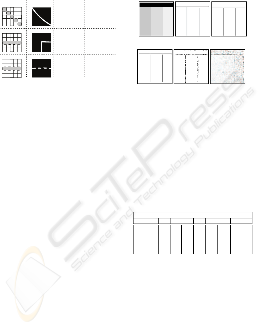
(a) Original image (b) Ideal edges (c) Intensity shift
(d) Shifted edges (e) Fragmented (f) Spurious edges
Figure 4: Typical grey-scale edge detection images used to
the show the inconsistencies inherent to edge comparison
metrics. Each image represents a common output edge de-
tection fault and is compared against the desired ideal image
(b) using all the discussed performance metrics (see Table 1
for the performance results).
Table 1: The results of using comparison metrics when to
common edge output images (Figure 4 c-f). Each image is
tested using the discussed comparison metrics against the
ground truth image (Figure 4b). PCM and CDM results
are shown over a defined pixel region of PCM0/CDM0=0,
PCM1/CDM1=1 and PCM2/CDM2=2. The first line of
the table indicates the results of comparing the ideal im-
age against itself with an ideal response expected from all
tests. Both the PCM and CDM metrics of edge evaluation
can give a falsely high response to extreme over-detection
of false edges caused by noise or texture (indicated in Bold-
face). Connectivity results are scaled between the ideal con-
nected edge =1 and disconnected edges = 0.
Evaluation of Edge Comparison Metrics
Image Name PCM0 PCM1 PCM2 CDM0 CDM1 GFOM Connectivity
Ideal 100 100 100 100 100 100 0.975
Intensity Shift 38.68 37.29 36.16 38.68 38.68 38.70 0.972
Shifted edges 33.19 33.81 34.32 33.91 33.81 22.70 0.956
Fragmented 36.66 53.5 53.93 36.66 36.74 35.50 0.075
Spurious edges 87.83 66.32 88.43 87.83 88.11 13.40 0.124
rectly located edges with an incorrect intensity level
(see Figure 4c). Correctly detected edges with a loca-
tion or shift error (see Figure 4d). Correctly located
edges that are broken or fragmented (see Figure 4e).
Noisy or spurious over-detected edges (see Figure 4).
Table 1 shows how all metrics perform accurately
if the edge height is comparable to the desired edge
height (see Figure 4b). Moreover if the detected edge
intensity is greater than the desired edge intensity, as
is common with some ranking statistical edge detec-
tors as in the work of (Svoboda et al., 2006), all per-
formance metrics reduce accordingly. This is not a
gauge of any inaccurate edge detection, but represents
a true correspondence of the actual grey-scale edge
height compared to the output detected edge inten-
A NOVEL PERFORMANCE METRIC FOR GREY-SCALE EDGE DETECTION
95
sity. If a small pixel shift is now introduced to the
results, as shown in Figure 4d then any results should
decrease with reference to this shift. Both PCM and
CDM allow for small shifts in pixel positions using
a user defined pixel mask to check for an optimal
match, and as such decrease as expected. GFOM uses
the distance transform to also allow for slight edge lo-
calisation errors and furthermore the performance is
seen to decrease in response to a shift (see Table 1).
If this detected edge becomes broken or frag-
mented as shown in Figure 4e, then a correct perfor-
mance metric should reduce accordingly. This is true
for both the CDM and GFOM metrics where the ob-
served performance is shown to reduce, however the
results clearly illustrate an inconsistency in the PCM
metric. With broken or fragmented edges the PCM
metric gives a higher performance value than it does
for an edge that is continuous (see Table 1). In addi-
tion to this, if the edge height in the image is a simi-
lar “strength” value to any spurious edges or noise in
the image, which can be common when assessing tex-
tured images, both the PCM and CDM metrics will
assume this to be a correctly detected edge. There-
fore with extreme over-detection of edges, as shown
in Figure 4f, both the PCM and CDM metrics give
a falsely high response (see Table 1). This problem
of incorrect performance for this over-detected (or
noisy) edge image is not matched by the new GFOM
which accurately measures this as the poorest result.
However, GFOM is not without its own faults.
GFOM takes every threshold level in the edge de-
tected image and checks the ground truth for an ex-
act match at that same threshold level, therefore it
will not tolerate edge intensity changes. The GFOM
technique can be adapted to avoid this problem by al-
lowing a ranged threshold comparison between both
images, however this would result in GFOM having
some of the same inconsistencies as highlighted for
both the PCM and CDM metrics. To avoid these prob-
lems all three performance metrics can be used in con-
junction allowing a consistency in the results unavail-
able with a single objective performance measure.
The results further showed how all the comparison
metrics were found to favour accurately located edges
over edges that, although accurate, have slight local-
isation errors (see Figure 4d). Moreover, a greater
edge performance measure could be awarded to an
edge that is accurately located but is badly fragmented
(see Figure 4e), against a poor response for an edge
that is continuous but has slight localisation errors
(see Table 1). In this situation it becomes important
to determine what is required by the edge detector.
If it can detect an accurate edge which is fragmented
or not continuous, then is this preferred over an edge
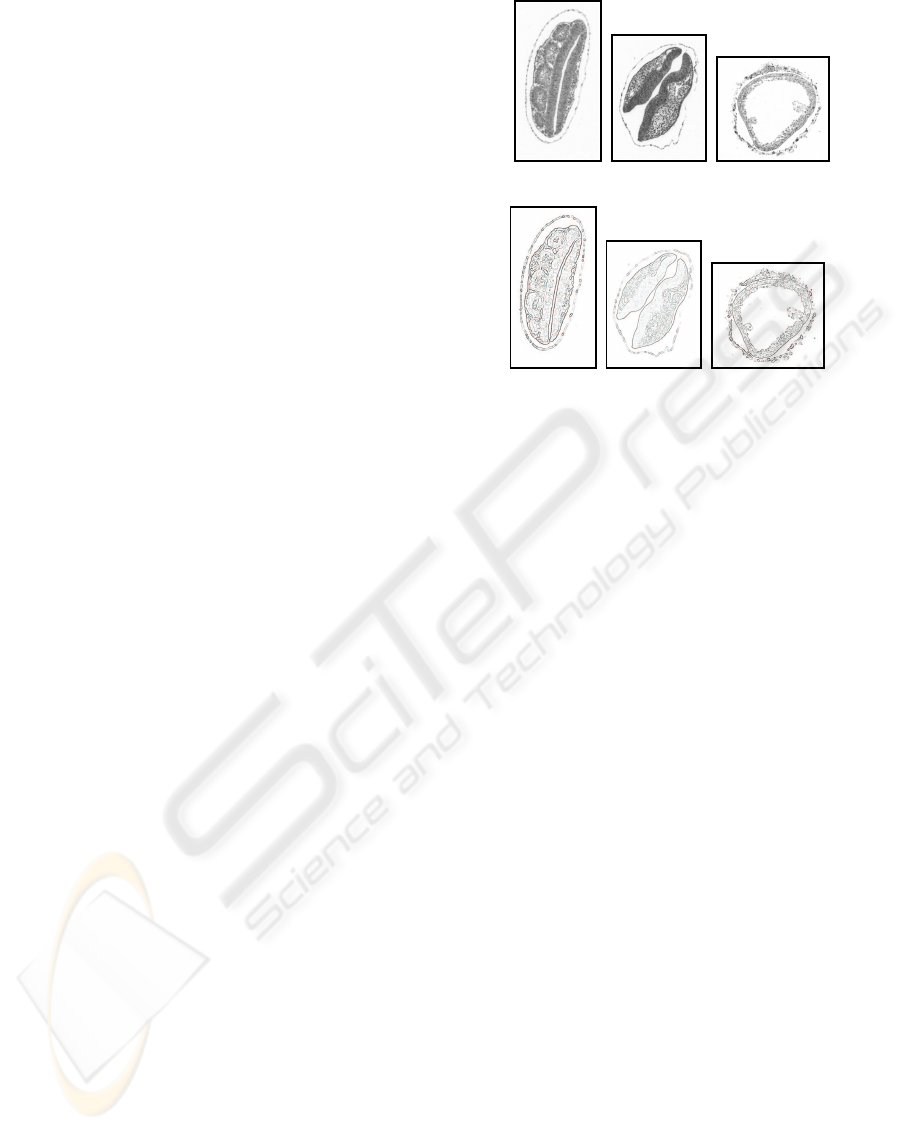
(a) ma3 (b) ma4 (c) ma74
(d) (e) (f)
Figure 5: A sample set of histological test images used in
the connectivity measurement, and the results after applying
the Canny edge detection with a σ = 2. Images courtesy of
the Edinburgh Mouse Atlas Project (EMAP).
shifted somewhat but is continuous and therefore un-
broken?
Many segmentation techniques, including those
of (Svoboda and Matula, 2003) and (Bowring et al.,
2004), require a continuous contour to accurately seg-
ment the objects. In this situation the localisation of
edges becomes less important and the connectivity of
edges is paramount. Therefore an accurate gauge of
the connectivity of the edge detection results can be
important as the metric for evaluation.
If we analyse the results for the connectivity of
edges (see Figure 3, Table 1 and Table 2) it is clear to
see the reduction in the connectivity measure awarded
to edges that are fragmented or broken. As previously
discussed the connectivity measure can be computed
over different sized pixel masks (see Table 2), there-
fore giving a different measure for each mask applied.
A larger connectivity mask will detect more variabil-
ity in the pixel points and give a greater sensitivity
to the results, however this can award sharp corners
or curvature in the image a lower connectivity value
(see Figure 3). Smaller connectivity masks will al-
low better performance for curvature and corners but
will be less sensitive to the changes (or breaks) in the
edge pixels. However, We can see that with a fixed
size pixel mask there is a consistent pattern in the
connectivity results for a uniform edge (connectivity
1.0), and non-uniform edge (connectivity 0.225) and
a corner or shape based edge (connectivity0.678), see
Figure 3.
VISAPP 2010 - International Conference on Computer Vision Theory and Applications
96

Table 2: Connectivity results for the Canny edge detector
across a selection of test images shown in Figure 5. Each
result is computed using a connectivity region mask of 5
(con.5),11 (con.11),15 (con.15) and 21 (con.21) pixels.
Connectivity Measurement
Image Canny (Con.5) Canny (Con.11) Canny (Con.15) Canny (con.21)
ma3 0.820 0.663 0.604 0.532
ma4 0.823 0.673 0.618 0.553
ma74 0.804 0.642 0.588 0.529
5 CONCLUSIONS
This paper discussed existing methods for evaluation
of greyscale edge detection and introduced new meth-
ods for edge detector evaluation. Initial results which
compared the common objective methods, showed
ambiguities in the evaluation. The Pixel Comparison
Metric (PCM) and Closest Distance Metric (CDM)
both showed inconsistencies when the edge detected
height is comparable to noise or false edges in the im-
age. It was further shown that if the detected edge
height is the same or a similar value to noise in the im-
age both metrics will give a falsely high performance
measure. Moreover, both the PCM and CDM metrics
were seen to give a greater response to over-detected
edges, than accurately located edges of different grey-
levels. This shows a bias in the results towards the
location of edges over the accuracy of edges.
The Greyscale Figure of Merit (GFOM) (an
adapted form of Pratt’s Figure of Merit) was then in-
troduced. The new GFOM measure can overcome
some of the inconsistencies of the PCM and CDM
metrics therefore allowing a more robust evaluation
of grey-scale edge detection against an ideal ground
truth. All the comparison metrics were found to
favour accurately located edges which were broken of
fragmented over edges that, although accurate, have
slight localisation errors. In this case a greater edge
performance measure could be awarded to an edge
that is accurately located but is badly fragmented,
against a poor response for an edge that is continu-
ous but has slight localisation errors.
To overcome this problem and aid in the evalua-
tion, a novel edge continuity measure was developed
and tested. This measure uses a unique pixel mask
applied to the edge image and assess the angle and
location of edges. The uniformity of the detected
edge pixels is then assessed and the connectivity of
the edge defined. This connectivity measure can be
used independently or in conjunction with the previ-
ously discussed metrics to give a robustness to the re-
sults currently unavailable with any single grey-scale
performance measure.
REFERENCES
Abdou, I, E. and Pratt, W, K. (1979). Quantitative design
and evaluation of enhancement/thresholding edge de-
tectors. Proceedings of the IEEE, 27(5): p. 753–763.
Boaventura, I. and Gonzaga, A. (2009). Method to evaluate
the performance of edge detector. In Workshops of
Sibgrapi 2009 - Posters.
Bowring, N. J., Guest, E., Twigg, P., Fan, Y., and Gadsby,
D. (2004). A new statistical method for edge detection
on textured and cluttered images. In 4
th
IASTED VIIP
Conf., pages 435–440.
Bowyer, K., Kranenburg, C., and Dougherty, S. (2001).
Edge detector evaluation using empirical roc curves.
CVIU, 84(1): p. 77–103.
Canny, J. (1986). A computational approach to edge detec-
tion. IEEE TPAMI, 8: p.679–698.
Fern´andez-Garc´ıa, N., Carmona-Poyato, A., Medina-
Carnicer, R., and Madrid-Cuevas, F. (2008). Auto-
matic generation of consensus ground truth for the
comparison of edge detection techniques. Image and
Vision Computing, 26(4):496 – 511.
Fesharaki, M. N. and Hellestrand, G. R. (1994). A new edge
detection algorithm based on a statistical approach. In
Proceedings of IEEE, pages 21–24.
Grigorescu, C., Petikov, N., and Westenberg, M. (2003).
Contour detection based on nonclassical receptive
field inhibition. IEEE TPAMI, 12(7): p. 729–739.
Heath, M., Sarkar, S., Sanocki, T., and Bowyer, K. (1996).
Comparison of edge detectors: A methodology and
initial study. CVIU, 69(1): p. 38–54.
Joshi, G. D. and Sivaswamy, J. (2006). A simple scheme
for contour detection. In Ranchordas, A., editor, 1st
INSTII Int. Conf. on VISAPP, pages 236–242. INSTII
Press – Portugal.
Pratt, W. K. (1978). Digital Image Processing. Wiley.
ISBN: 0-471-37407-5.
Prieto Segui, M. and Allen, A. (2003). A similarity metric
for edge images. IEEE TPAMI, 25(10): p. 1265–1273.
Svoboda, D. and Matula, P. (2003). Tissue reconstruction
based on deformation of dual simplex meshes. In
I. Nystr¨om, G. S. di Baja, S. S., editor, DGCI, vol-
ume 2886 of LNCS, pages 524–533. Springer – Berlin,
Heidelberg, New York.
Svoboda, D., Williams, I., Bowring, N., and Guest, E.
(2006). Statistical techniques for edge detection in
histological images. In 1
st
Int. Conf. on VISAPP,
pages 457–462. INSTICC Press – Portugal.
ˇ
Sonka, M., Hlav´aˇc, V., and Boyle, R. (1986). Image Pro-
cessing Analysis and Machine Vision. Chapman and
Hall Publishing.
Zhu, Q. (1995). Efficient evaluations of edge connectivity
and width uniformity. Image and Vision Computing,
14(1): p. 21–34.
A NOVEL PERFORMANCE METRIC FOR GREY-SCALE EDGE DETECTION
97
