
AN EMPIRICAL EVALUATION OF A GPU RADIOSITY SOLVER
Guenter Wallner
Institute for Art and Technology, University of Applied Arts, Oskar Kokoschka Platz 2, Vienna, Austria
Keywords:
Global illumination, Radiosity, GPU programming, Projections.
Abstract:
This paper presents an empirical evaluation of a GPU radiosity solver which was described in the authors pre-
vious work. The implementation is evaluated in regard to rendering times in comparision with a classical CPU
implementation. Results show that the GPU implementation outperforms the CPU algorithm in most cases,
most importantly, in cases where the number of radiosity elements is high. Furthermore, the impact of the
projection – which is used for determining the visibility – on the quality of the rendering is assessed. Results
gained with a hemispherical projection performed in a vertex shader and with a real non-linear hemispherical
projection are compared against the results of the hemicube method. Based on the results of the evaluation,
possible improvements for further research are pointed out.
1 INTRODUCTION
Radiosity has been and is still a widely used tech-
nique to simulate diffuse interreflections in three-
dimensional scenes. Radiosity methods were first de-
veloped in the field of heat transfer and in 1984 gener-
alized for computer graphics by (Goral et al., 1984).
Since then, many variations of the original formula-
tion have been proposed, leading to a rich body of
literature available on this topic. See e.g. the book by
(Cohen and Wallace, 1995) for a good overview of the
field. An extensive comparison of different radiosity
algorithms can be found in (Willmott and Heckbert,
1997).
In recent years research on GPU accelerated ra-
diosity algorithms intensified. (Nielsen and Chris-
tensen, 2002) used hardware texture mapping to ac-
celerate the hemicube method and (Carr et al., 2003)
were the first to utilize floating point textures to store
the radiosity values. (Coombe et al., 2003; Coombe
and Harris, 2005) described the first radiosity solver
for planar quadrilaterals that performed all steps on
programmable graphics hardware. In (Wallner, 2008)
we described a GPU radiosity system for arbitrary tri-
angular meshes which built upon the work mentioned
above.
The purpose of this paper is twofold. First, pre-
senting the results of an empirical evaluation of our
GPU radiosity solver in regard to rendering times and
on how the projection used for creating the visibility
map effects the final image quality and secondly to
point out possible improvements for further develop-
ment.
The reminder of this paper is structuredas follows.
Section 2 gives a short overview of the various steps
of the radiosity implementation. In Section 3 timings
for the individual steps are given for a set of sample
scenes. Section 4 compares rendering times with a
CPU implementation and the impact of the applied
projection on the quality of the result is discussed in
Section 5. The paper is concluded in Section 6.
2 OVERVIEW
This section gives a short overview of the main steps
performed by the progressive radiosity solver, which
are as follows:
Preprocess. In the preprocess two textures – which
store radiosity and residual energy values – are gener-
ated for each triangle which themselves are placed in
larger lightmaps to reduce texture switching later in
the process. Furthermore the required framebuffers,
auxiliary textures and other OpenGL related resources
are allocated.
Next Shooter Selection. In this step a mipmap pyra-
mid is constructed for each residual lightmap until
each triangle is represented by a single texel. These
values are read back to the CPU and the triangle with
the highest value is selected as next shooter. This step
is performed using a ping-pong technique. Standard
225
Wallner G. (2010).
AN EMPIRICAL EVALUATION OF A GPU RADIOSITY SOLVER.
In Proceedings of the International Conference on Computer Graphics Theory and Applications, pages 225-232
DOI: 10.5220/0002822202250232
Copyright
c
SciTePress
OpenGL mipmapping cannot be used because texels
not occupied by the triangle have to be omitted. For
the shooter, four textures – world position map, nor-
mal map, color map and intensity map – are gener-
ated which are necessary for calculation of the energy
transport. Shooting is performed from a user-defined
mipmap level of these textures. This way the accuracy
and speed of the calculation can be influenced.
Render Visibility Texture. To determine the visible
surfaces a hemicube projection, a stereographic pro-
jection (performed in the vertex shader) or the non-
linear hemisphere projection by Gascuel et al. (Gas-
cuel et al., 2008) is used to generate a depth texture
from the shooter’s viewpoint.
Adaptive Subdivision. If adaptive subdivision is en-
abled, occlusion queries are used during rendering
of the visibility texture, to check on which triangles
shadow boundaries are located. If the ratio between
visible texels and texels in shadow is between certain
thresholds and the maximum subdivision level is not
reached, the triangle is subdivided.
Update Receivers. Visible or partially visible trian-
gles (determined by checking the outcome of an oc-
clusion query) are back-projected into the visibility
texture and their depth values are compared against
the stored values. If they match, then the radiosity
and residual maps are updated accordingly. Calcula-
tion of the form factors is therefore performed in this
step.
Postprocess. Because the rasterized triangles cannot
be directly used for texturing – polygon rasterization
rules differ from texture sampling rules (Segal and
Akeley, 2003) – missing values are linearly interpo-
lated in a shader. This step is performed once after
the progressive radiosity solver has finished.
The system was implemented in C++ and OpenGL
with the shaders written in Cg. For a more in-depth
description of the solver refer to (Wallner, 2008) and
(Wallner, 2009). In the remainder of this paper we
will refer to one cycle of the progressive radiosity
solver as an iteration in contrast to a shooting step
from a single texel of the mipmap texture of the se-
lected shooting triangle.
3 PERFORMANCE
To assess the time spent on the above mentioned steps
we used four different test scenes, which vary in the
number of triangles and light sources. All the mea-
surements in this work were taken on an Intel Core2
CPU with 2.13 GHz, 3.5 GB RAM with a Geforce
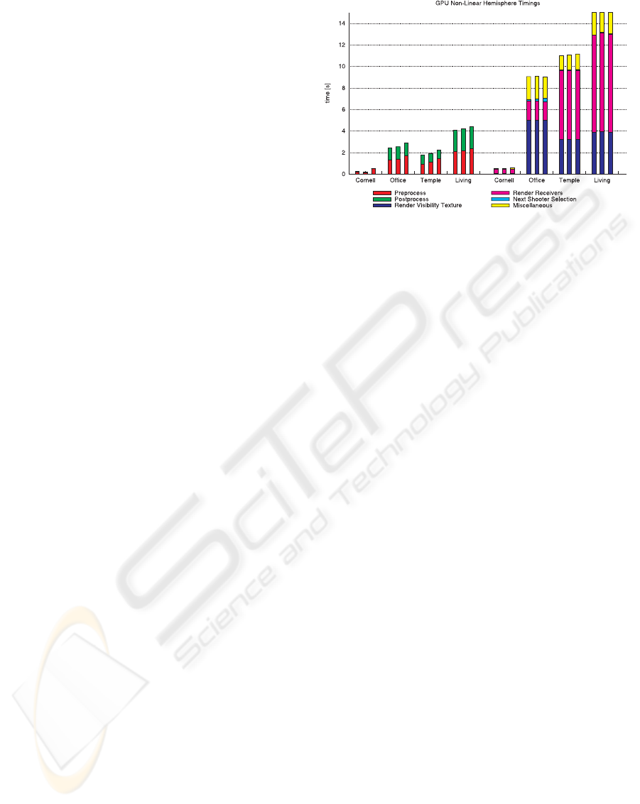
Figure 1: Time spent on different steps of the radiosity com-
putation for different scenes with increasing triangle count
from left to right (each time for three different resolutions
as listed in Table 1) for 32 shootings. The left group shows
steps executed once, whereas the steps in the right side are
performed multiple times.
8800GTS with 640MB DDR3 Ram. The scenes (ex-
cept the Cornell Box) are shown in Figure 2 whereas
Figure 1 depicts the measurements in case of the non-
linear hemisphere. The hemicube is rendered with a
single-pass cubemap geometry shader with multiple
attached layers. This has the advantage that an oc-
clusion query (required for subdivision and visibility
purposes) counts all rasterized fragments over all at-
tached layers, which makes management of them eas-
ier than with a multi-pass approach. Performing the
hemispherical projection in the vertex shader reduces
the time needed for the creation of the visibility tex-
ture by about 30 to 55 percent. However, if the scene
is not carefully triangulated the hemispherical projec-
tion can lead to severe artifacts (see Section 5).
Time for rendering the visibility texture depends
solely on the number of triangles, whereas the time
needed for the next shooter selection depends on the
number of lightmaps and the ratio of the lightmap size
to the stored texture size. Updating the receivers is
by far the most time consuming function in the pro-
cess. In this regard the biggest restriction is currently
that GPUs do not allow to simultaneously read from
and write to the same position in a texture. There-
fore it is necessary to render the new radiosity and
residual maps to intermediate textures and copy them
afterward to the correct position in the lightmap. An-
other possibility would be to maintain two textures
for storing the radiosity and further two for the resid-
ual energy and use them in a ping pong technique.
We rejected this method because it would double the
memory requirements.
The cost for the post-process primarily depends on
the number of triangles. To reduce the required time
GRAPP 2010 - International Conference on Computer Graphics Theory and Applications
226
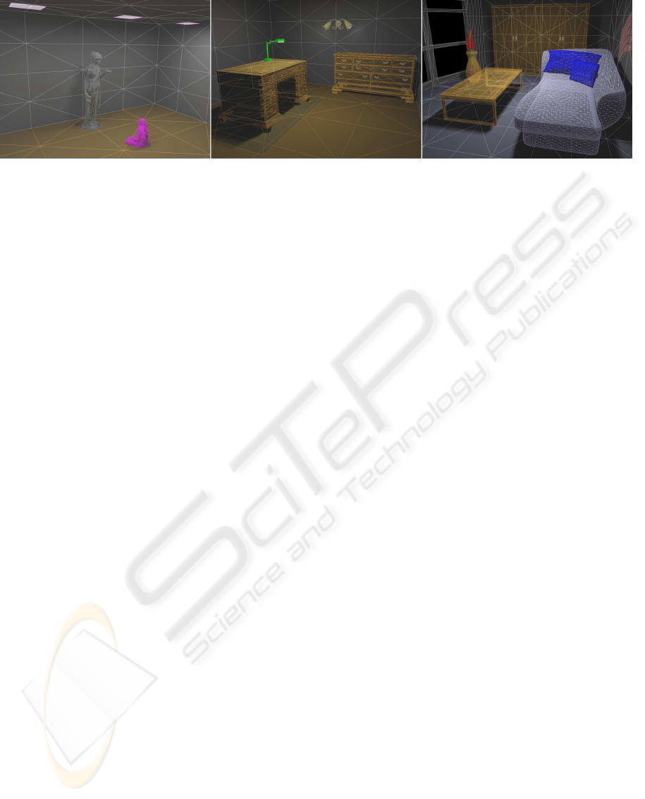
Figure 2: These are the different test scenes used for the analysis. From left to right: A temple with three light sources (6
triangles), an old office with 24 light emitting triangles distributed over four light sources and a more modern room with one
light source (2 triangles).
for the post-process we initially hoped that with con-
servative rasterization (Hasselgren et al., 2005) the
textures could be directly used for nearest-neighbor
texture sampling. This, however, proved to be diffi-
cult since the geometry itself is inflated and therefore
the interpolation of normals and other attributes is al-
tered, which inevitable leads to discontinuities at the
boundaries of the triangles. It is clear that the cost of
the pre- and post-process amortizes with increasing
number of performed iterations.
4 CPU COMPARISON
To compare the performance of our solution with
a software implementation we chose the radiosity
solver of the open source software Blender 2.48a
(Blender Foundation, b). We opted for Blender be-
cause it is freely available and the settings of its ra-
diosity system can be closely matched with the ones
from our implementation. The hemicube resolution
was set to 512× 512 and in case of the stereographic
projection a 2048 × 2048 resolution was used. The
calculation was terminated after a fix number of iter-
ations. We have preferred iterations over convergence
because the time needed to reach a certain conver-
gence depends on the mipmap level chosen for shoot-
ing in our method. Ensuring the same number of it-
erations between the CPU and GPU implementation
would therefore be hard to control. Adaptive sub-
division was disabled in our implementation, since
Blender performs no adaptive refinement (Blender
Foundation, a). Table 1 lists the timings for differ-
ent scenes. For the test scenes our GPU implemen-
tation achieved speed-ups of up to 46 times. In con-
trast to the CPU implementation, the calculation time
is nearly unaffected by the number of elements (that
is, the resolution of the radiosity maps). Calculation
time on the GPU is mostly determined by the num-
ber of triangles in the scene, since for each triangle a
texture copy is performed during update of the radios-
ity and residual textures. The non-linear hemisphere
projection achieved about 20 to 40 percent faster ren-
dering times than the hemicube method.
In cases where the number of elements is very low
the CPU outperforms the GPU, as it is e.g. the case
in the low resolution temple scene. In such scenarios
the cost of the initial pre-process of transferring the
data to the GPU, the allocation of resources and the
required post-process are high compared to the actual
processing time.
5 PROJECTIONS
In this section the influence of the projection utilized
for creating the visibility map on the visual quality of
the result is discussed. The classical method for deter-
mining visibility from a given point is the hemicube,
as proposed by (Cohen and Greenberg, 1985). The
drawback is that the scene has to be rendering five
times to project all possible receiving surfaces onto
the individual sides of the hemicube. Since visibility
determination is a frequently performed task in the
radiosity process, it is beneficial to reduce rendering
time. (Beran-Koehn and Pavicic, 1991; Beran-Koehn
and Pavicic, 1992) used a cubic tetrahedron instead a
hemicube, thereby reducing the number of projecting
planes to three. The number of projections were fur-
ther reduced by using a single-plane projection (e.g.
(Sillion and Puech, 1989)) or hemisphere (base) pro-
jections which, to our knowledge, were first proposed
by (Spencer, 1992). In this case the projection is a
simple normalization process and clipping can sim-
ply be performed against the base plane of the hemi-
sphere. To ensure an accurate projection, (Spencer,
1992) calculates the degree of the arc between pairs of
points projected onto the hemisphere basis and uses
this value to calculate intermediate points along the
edge. A scan-conversion algorithm is then used to
AN EMPIRICAL EVALUATION OF A GPU RADIOSITY SOLVER
227
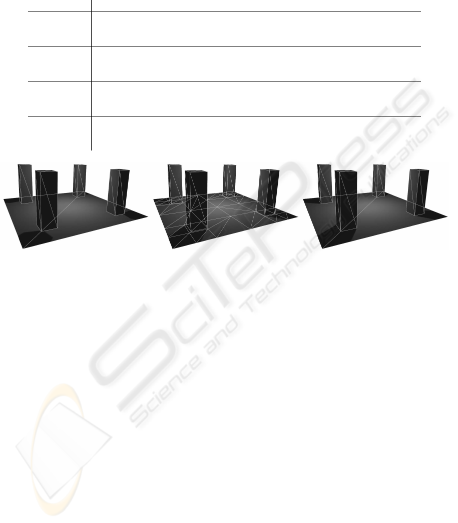
Table 1: Performance comparison between a CPU radiosity solver t
cpu
and our implementation (t
gpu,cube
for the hemicube
and t
gpu,sphere
for the non-linear hemispherical projection with the speed-up in brackets). The number of elements is given in
the columns n
cpu
and n
gpu
. Because our method uses power-of-two textures the number of elements differ, nonetheless we
tried to match them as closely as possible. n
t
lists the number of triangles and s the number of shootings.
Scene
s n
t
n
cpu
n
gpu
t
cpu
[s] t
gpu,sphere
[s] t
gpu,cube
[s]
cbox
low
32 258 9248 11802 1.97 0.79 (× 2.5) 1.15 (× 1.7)
cbox
medium
32 258 82976 94750 5.69 0.75 (× 7.6) 1.13 (× 5.0)
cbox
high
32 258 1026464 1115126 54.19 1.17 (× 46.3) 1.48 (× 36.6)
temple
low
24 15872 117248 126078 5.60 9.74 (× 0.6) 12.58 (× 0.4)
temple
medium
24 15872 507320 516312 18.27 9.92 (× 1.8) 12.72 (× 1.4)
temple
high
24 15872 1741208 2074242 53.13 10.03 (× 5.3) 13.18 (× 4.0)
office
low
96 21704 264081 254572 36.17 18.46 (× 1.3) 42.46 (× 0.8)
office
medium
96 21704 747375 854341 84.62 18.03 (× 4.7) 42.44 (× 2.0)
office
high
96 21704 1846137 1843771 202.54 18.73 (× 10.8) 43.03 (× 4.7)
living
low
32 38147 474744 472317 37.23 20.18 (× 1.8) 33.10 (× 1.1)
living
medium
32 38147 861540 866330 44.41 20.05 (× 2.2) 33.24 (× 1.3)
living
high
32 38147 1570884 1612067 73.88 20.61 (× 3.6) 33.45 (× 2.2)
Figure 3: Left: Incorrect shadows as the result of erroneous visibility information due to the hemispherical projection. Mid-
dle: Adaptively tessellating the surface around the shadow boundary reduces the errors enormously. Right: Solution of the
hemicube method on the original mesh.
determine the area covered by the projected surface
element. The method, however, fails to remove hid-
den surfaces in certain cases, which was resolved by
(Doi and Takayuki, 1998) by subdividing the surface
– based on a solid angle criterion – into smaller trian-
gles instead of using edge-subdivision. Hemisphere
projections are currently frequently performed in ver-
tex shaders on programmable GPUs, e.g. (Coombe
et al., 2003; Barsi and Jakab, 2004; Coombe and Har-
ris, 2005). However, since only vertices are affected
by the hemispherical projection – straight edges are
mapped to straight edges instead of elliptical seg-
ments – errors are introduced. To approximate the
correct curvature, one solution would be to tessellate
the surfaces finely enough, as e.g. done in (Coombe
et al., 2003). This increases the triangle count of the
scene considerably and consequently rendering times.
Assuming that no two surfaces overlap, it is sufficient
to perform the back-projection in the vertex shader
as done in (Wallner, 2008; Barsi and Jakab, 2004).
However, if surfaces overlap, the relative position in-
formation between the surfaces is distorted in the pro-
jection which results in more or less incorrect shadow
boundaries. Figure 3 illustrates this problem. How-
ever, adaptive subdivision methods (see e.g. (Cohen
and Wallace, 1995)) to improve the accuracy of the
radiosity solution in areas of high-frequency lighting
also reduce the errors due to the hemisphere projec-
tion significantly. Therefore it seems to be unneces-
sary to uniformly tessellate the mesh just for the pur-
pose of the projection.
A further problem in conjunction with too coarse
meshes is that the projection of some triangles may
be extremely deformed and therefore are not rendered
at all, although they should be. These triangles are
misleadingly considered not visible and thus omitted
during the radiosity exchange. Figure 4 shows an ex-
ample where this is the case. This problem is intrin-
sic to hemispherical projections because distortions
increase for directions further from the viewing di-
rection. Using a paraboloid projection would reduce
these errors since the sampling rate is more uniform
than in the spherical case (see (Heidrich and Seidel,
1998)). However, the actual problem remains.
(Kautz et al., 2004) proposed a method for spher-
ical rasterization, by defining a plane through each
edge of the triangle and the projection center. Then
a pixel is considered inside the projected image of the
GRAPP 2010 - International Conference on Computer Graphics Theory and Applications
228
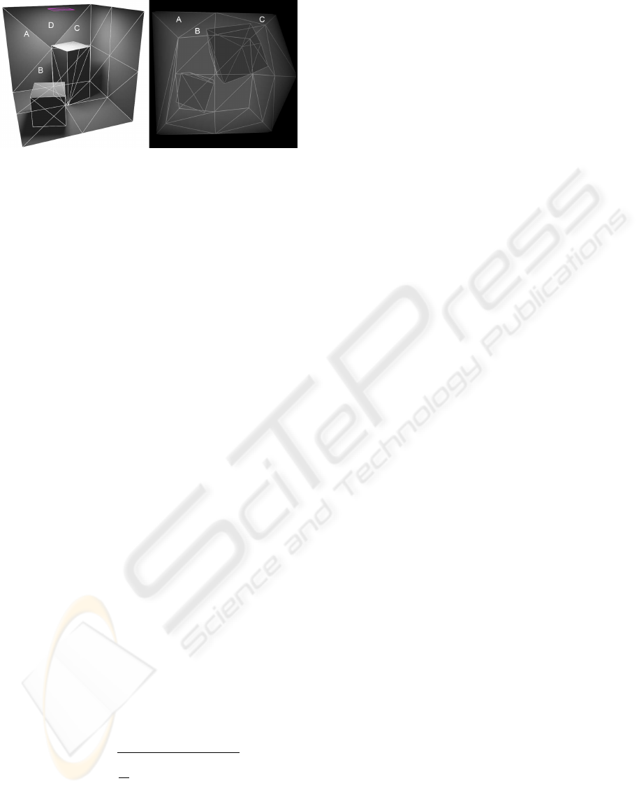
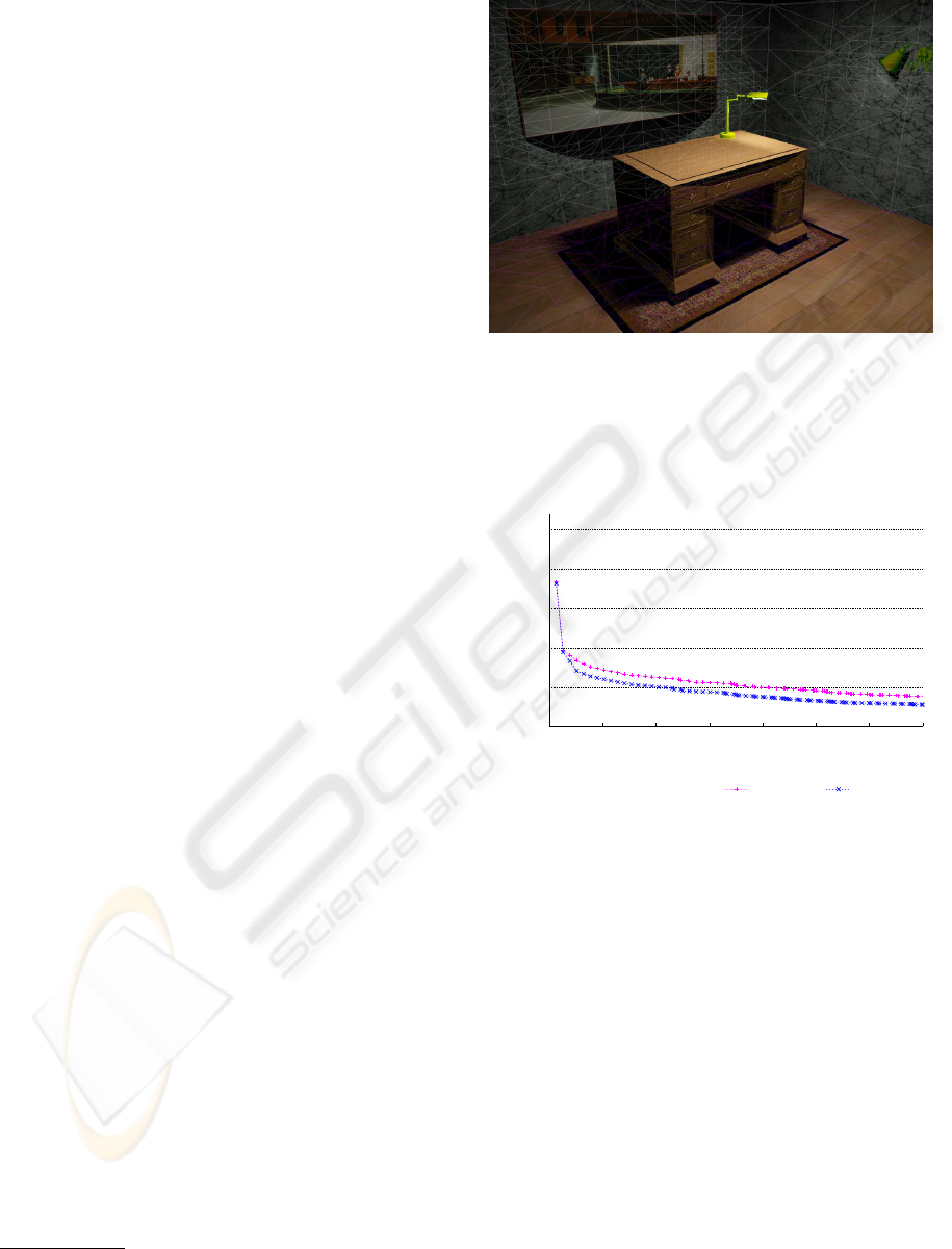
Figure 4: Triangle D at the back wall is sometimes consid-
ered as not visible, since its projection is that much distorted
that it is not rendered during creation of the visibility tex-
ture (shown on the right side with a wireframe overlay to
better show the connection to the scene).
triangle if the corresponding point on the hemi-
sphere is above all three planes. Because they were
only concerned with low-resolution visibility masks,
they were able to precompute a lookup table of bit-
masks for a discrete set of planes. In our case this
method is not feasible because the visibility map is
too large. We therefore implemented the recently
published method by Gascuel et al. (Gascuel et al.,
2008) to calculate non-linear projections with a sin-
gle projection center on graphics hardware. Their
algorithm consists of two steps. First, a bounding
primitive for each triangle is computed in a geome-
try shader. Second, each fragment is tested whether it
is inside the original triangle or not (in which case the
fragment is discarded).
5.1 Quantitative Analysis
To quantitatively assess the errors introduced by the
hemispherical projection, different scenes were ren-
dered with this projection and with the hemicube
method. This was done three times for each scene,
once with the original geometry, once with adap-
tive subdivision and once with a regularly refined
mesh. Each time the resulting lightmaps were read-
back from the GPU and compared with the root mean
square (RMS) metric. Calculating the RMS on the
lightmaps has the advantage that the estimated error
is view-independent. For N lightmaps of size X × Y
the RMS is given by
RMS =
v
u
u
t
1
m
N
∑
n=1
X
∑
x=1
Y
∑
y=1
|v
n
xy
| · a
n
xy
(1)
where v
n
xy
is the color-difference vector between
the R, G, and B values at pixel position (x, y) between
the n-th lightmap produced by hemispheical projec-
tion and the corresponding lightmap computed with
the hemicube method.
Pixels which do not belong to a triangle in the
lightmap are neglected by multiplication with the the
alpha-value a
n
xy
at the current position, which is either
1 or 0 if the pixel is occupied by a triangle or not.
This is necessary because such pixels are not part of
the solution and would only dilute the RMS value. m
is therefore the number of occupied pixels (a = 1) in
all lightmaps. Since the result of the adaptive subdivi-
sion can vary between the hemicube and hemisphere
solution, the result of the adaptive subdivision gained
by the hemisphere solution was used for the hemicube
method. Table 2 lists these root mean square values
for two different scenes. In this case we did not keep
the iterations fixed but rather aborted the calculation
once a given convergence threshold was reached. The
measurements were performed for different subdivi-
sion levels with different texture sizes. For the origi-
nal mesh 256× 256 textures were used, which yields
a resolution of 512× 512 for a quad. This means the
regular subdivision with level 3 and a texture size of
64 matches the original resolution most closely.
First of all, the RMS-error in case of the Cornell
Box is higher throughout than for the column scene
since the light source is much closer to the scene ge-
ometry. As is apparent from Table 2 (and as expected)
a regular subdivision reduces the RMS error quite sig-
nificantly, up to 13 times. This is the case even if
the overall resolution over a non-subdivided quad is
smaller than the 512× 512 texels used on the original
geometry (e.g. using a regular subdivision with level
3 and texture size 32 yields still a better result than
achieved with the original mesh). However, a regu-
larly subdivided mesh also increases rendering times
considerably. This is, on the one hand, due to the in-
creased number of triangles and, on the other hand –
which may not be obvious at first – due to the fact
that more triangles covering the same area means less
energy per triangle which in turn requires more itera-
tions to reach a given convergence threshold.
We are looking into two options to further de-
crease rendering times:
1. Currently a single texture size is used for the
whole mesh (although sizes can vary between
meshes), which may be suboptimal since triangles
sizes can vary over the mesh. In this sense, it may
be promising to base the texture resolution on tri-
angle size. However, first results showed inter-
polation artifacts along triangle edges due to the
different resolutions.
2. The mipmap level used for shooting may be de-
cided adaptively rather than being fixed for the
whole calculation. The level may also depend
on the average energy of the current shooting tri-
AN EMPIRICAL EVALUATION OF A GPU RADIOSITY SOLVER
229
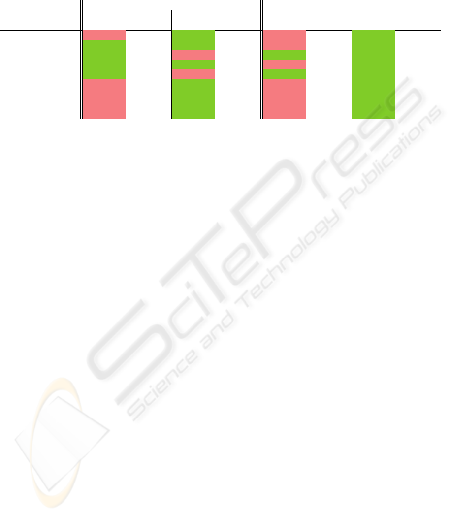
Table 2: RMS error for the hemispherical projection (compared to the hemicube solution). The table lists the type of subdi-
vision type
sub
which is either no (no subdivision), adapt (adaptive subdivision) or reg (regular refinement), and the level of
subdivision. The texture size is given in column size and the rendering time is listed in column t. If a solution is considered
perceptually indistinguishable from the hemicube solution it is highlighted in green, otherwise in red.
Columns Cornell Box
hemisphere non-linear hemisphere hemisphere non-linear hemisphere
type
sub
level size RMS t[s] RMS t[s] RMS t[s] RMS t[s]
no 0 256 0.001745 1.836580 0.000279 2.191166 0.005399 1.543515 0.001286 2.265481
adapt 3 32
0.002047 0.997896 0.000953 2.134127 0.005451 3.731590 0.007660 4.174523
reg 3 32
0.000331 9.142668 0.000104 10.184814 0.001772 14.641043 0.000458 20.789242
adapt 3 64
0.000789 1.179061 0.000397 2.295658 0.002147 5.382289 0.002708 4.373851
reg 3 64
0.000133 28.540912 0.000057 29.953424 0.000766 79.602470 0.000237 97.384330
adapt 2 32
0.003907 0.903491 0.001434 1.968630 0.040701 1.466952 0.011807 3.244810
reg 2 32
0.001287 2.791759 0.000457 3.137670 0.004473 2.777053 0.001942 4.120059
adapt 2 64
0.001726 1.004140 0.000576 2.064948 0.020571 1.644687 0.004213 3.477550
reg 2 64
0.000591 3.272110 0.000187 3.731351 0.001784 4.809930 0.000709 7.562907
angle or on the global ambient radiosity term.
This would make sense, since triangles with less
residual energy make a smaller contribution to the
overall image. In the same way the most notice-
able contributions are being made at the beginning
of the progressive radiosity algorithm.
However, as evident from Table 2, the RMS error
can be already reduced by using adaptive subdivision
which simultaneously keeps rendering times low. In
fact, it reduces the most noticeable errors near shadow
boundaries as depicted in Figure 3. In some cases
rendering times are even lower than with the original
geometry. This is the case because lower resolutions
were used, meaning that there are less shootings from
a single triangle. In contrast to the regular subdivi-
sion, areas with no shadow boundaries (which there-
fore have higher residual energies on average) are not
refined in the same extent which in turn means that the
energy is not distributed over that many triangles and
therefore the number of iterations is not increased by
the same extent as is the case for regular subdivision.
There is a special case in the results which may
need further explanation. In case of the three times
adaptively subdivided Cornell Box with a texture res-
olution of 64× 64, rendering with the hemispherical
projection is slower than with the non-linear hemi-
sphere projection. As described in Section 2 our sub-
division method is based on the ratio between visible
and occluded pixels of a triangle. This information
is gained from the visibility texture. In this partic-
ular example the visibility texture of the hemisphere
projection gives incorrect information about shadow
boundaries, yielding more subdivisions than actually
necessary. In contrast, the non-linear hemispherical
projection of Gascuel et al. (Gascuel et al., 2008)
gives much better RMS values. The remaining dif-
ferences are presumable caused by different resolu-
tions used for the hemicube and hemispherical visi-
bility maps and due to the increasing distortions to-
ward the perimeter. It should be pointed out that the
non-linear hemispherical projection may suffer from
the same sampling problems as the hemispherical pro-
jection: small triangles may be not visible in the pro-
jected image.
5.2 Perceptual Analysis
Although the RMS values quantitatively show the im-
provement in image quality, they do not reflect if the
improvement is sufficient enough to avoid visual dif-
ferences noticeable by a human observer. Therefore
we used the perceptual metric of Yee (Yee, 2004)
to assess if there are perceptual differences between
the hemicube method and the hemispherical varia-
tions. We have chosen this method because an im-
plementation is publicly available. The algorithm re-
quires some user defined parameters for which the
standard values were used, except for the field-of-
view angle which was set to 37
◦
(assuming an ob-
server looking from 0.5m at a 17” display). An image
was considered different if more than 100 pixels (ap-
prox. 1.2% of the image) were perceptually different.
Since it does not make sense to apply the metric on
the lightmaps themselves, we rendered five different
views of each scene and applied the metric to the tone-
mapped result. Progressive radiosity was turned off
because it can change the shooting order and there-
fore can lead to slightly different results. A solution
was considered to have no difference only if all of the
views were indistinguishable.
The perceptual metric revealed two problems.
First, if silhouette edges are at glancing angles in re-
gard to the projection center, some texels around this
edge may be incorrectly classified as in-shadow if one
of the two hemispherical projections is used. This
seems to be caused by the discretized nature of the
visibility map in conjunction with limited depth pre-
cision. Sampling the visibility map at the neighboring
GRAPP 2010 - International Conference on Computer Graphics Theory and Applications
230
texels reduced these problems significantly. Indistin-
guishable solutions after this modification are high-
lighted green in Table 2, otherwise they have a red
background. The two red entries for the non-linear
hemispherical projection are caused by the formerly
described problem, that surfaces may not be visible
in the visibility map due to distortions. Second, if
a hemispherical projection is used, shadows may be
smaller or larger than they should be. This was ev-
ident in some results because it proved to be inade-
quate to subdivide only surface elements which are
partly in shadow as implemented in our adaption sub-
division algorithm. Rather is it necessary to subdi-
vide shadow casting surfaces as well, otherwise their
boundaries do not reproduce the circular arc accu-
rately enough (the surface being smaller or larger and
therefore allowing more respectively less light to im-
pinge on the receiving surfaces). An example where
this problem leads to larger shadows is shown in Fig-
ure 5. This issue may be resolved by adaptively tes-
sellating the triangles during creation of the visibility
map with a geometry shader. However, this subdivi-
sion also has to be considered during back-projection
of the individual surfaces. We will look into this issue
as part of our future work.
Finally, it should be pointed out that errors in the
visibility information may not only affect the image
quality of the solution but even the convergence of
the radiosity process. In some rare cases we even
observed longer rendering times with the hemisphere
projection as with the hemicube method, since many
areas are incorrectly considered to be in shadow
1
.
Figure 6 compares the convergence of a scene, where
the errors caused by the stereographic projection in-
creased the number of shootings from 3514 to 4106
and consequently the rendering time from 182.06 sec-
onds to 192.93 seconds.
6 CONCLUSIONS
In this paper we presented an analysis of our GPU
radiosity solver. Measurements showed that the per-
formance is mostly independent of the dimensions of
the radiosity maps (if the mipmap level for shooting
is adjusted accordingly to keep the number of shoot-
ings identical). The implementation would benefit if
reading from and writing to the same texture location
were possible. In most cases the GPU implementa-
tion is considerably faster than the CPU implementa-
tion. The cost for setting up the required OpenGL re-
1
This mostly occurs near the perimeter of the hemi-
sphere where distortions are very common.
Figure 5: A typical problem caused by hemispherical pro-
jection. Although the shadow receiving surface (the wall) is
tessellated highly enough, the shadow caster (the picture) is
not. The bottom edge of the picture which is responsible for
the shadow is a straight line in the projection and therefore
leads to an elliptical shadow.
0
500
1000
1500
2000
2500
0
500
1000
1500
2000
2500
3000
3500
Residual Energy
Shootings
Living Room, Convergence
stereographic
hemicube
Figure 6: Comparison of the convergence for the first 3500
shootings between hemisphere and hemicube projection.
Subdivision was disabled in both cases to highlight the ef-
fect of errors in the visibility information on the conver-
gence. Note the steep decrease near the beginning in the
case of the hemicube, which is not the case with the hemi-
spherical projection.
sources relativises with increasing number of radios-
ity elements and iterations.
Although a hemispherical projection performed in
the vertex shader accelerates the creation of the visi-
bility textures, it has several drawbacks which have an
impact on the quality of the result. First, the relative
position information of overlapping surfaces is dis-
torted, leading to incorrect shadow boundaries. Sec-
ond, extreme deformations may lead to incorrect vis-
ibility classification, misleadingly considering com-
plete surfaces as not visible. Third, if the shadow
boundaries are incorrect due to erroneous visibility
information caused by the hemispherical projection,
AN EMPIRICAL EVALUATION OF A GPU RADIOSITY SOLVER
231

then the subdivision method may unnecessarily sub-
divide triangles which in turn leads to longer render-
ing times. A real non-linear projection overcomes
almost all of these drawbacks and at the same time
decreases rendering times considerably. However,
the non-linear projection still exhibits some distortion
and sampling problems which are intrinsic to hemi-
spherical projections. Finally, we proposed possible
solutions to problems which were revealed during the
evaluation and which will be part of our future work.
REFERENCES
Barsi, A. and Jakab, G. (2004). Stream processing in global
illumination. Proceedings of 8th Central European
Seminar on Computer Graphics.
Beran-Koehn, J. C. and Pavicic, M. J. (1991). A cubic tetra-
hedral adaptation of the hemicube algorithm. Graphic
Gems II, pages 299–302.
Beran-Koehn, J. C. and Pavicic, M. J. (1992). Delta form-
factor calculation for the cubic tetrahedral algorithm.
Graphics Gems III, pages 324–328.
Blender Foundation. Blender manual. available on-
line:
http://wiki.blender.org/index.php/Doc:
Manual
.
Blender Foundation. Blender product website.
http://
www.blender.org
.
Carr, N. A., Hall, J. D., and Hart, J. C. (2003). Gpu
algorithms for radiosity and subsurface scattering.
In HWWS ’03: Proceedings of the ACM SIG-
GRAPH/EUROGRAPHICS conference on Graphics
hardware, pages 51–59, Aire-la-Ville, Switzerland.
Eurographics Association.
Cohen, M. F. and Greenberg, D. P. (1985). The hemi-cube:
a radiosity solution for complex environments. In
SIGGRAPH ’85: Proceedings of the 12th annual con-
ference on Computer graphics and interactive tech-
niques, pages 31–40, New York, NY, USA. ACM
Press.
Cohen, M. F. and Wallace, J. R. (1995). Radiosity and Re-
alistic Image Synthesis. Morgan Kaufmann.
Coombe, G. and Harris, M. (2005). Global illumination
using progressive refinement radiosity. In GPU Gems
2, pages 635–647. Addison-Wesley Professional.
Coombe, G., Harris, M., and Lastra, A. (2003). Radios-
ity on graphics hardware. Technical report, Univ. of
North Carolina, UNC TR03-020.
Doi, A. and Takayuki, I. (1998). Accelerating radiosity so-
lutions through the use of hemisphere-base formfactor
calculation. The Journal of Visualization and Com-
puter Animation, 9:3–15.
Gascuel, J.-D., Holzschuch, N., Fournier, G., and P
´
eroche,
B. (2008). Fast non-linear projections using graphics
hardware. In I3D ’08: Proceedings of the 2008 sym-
posium on Interactive 3D graphics and games, pages
107–114, New York, NY, USA. ACM.
Goral, C. M., Torrance, K. E., Greenberg, D. P., and Bat-
taile, B. (1984). Modeling the interaction of light
between diffuse surfaces. In SIGGRAPH ’84: Pro-
ceedings of the 11th annual conference on Computer
graphics and interactive techniques, pages 213–222,
New York, NY, USA. ACM Press.
Hasselgren, J., Akenine-M
¨
oller, T., and Ohlsson, L. (2005).
Conservative rasterization. In GPU Gems 2. Adison-
Wesley.
Heidrich, W. and Seidel, H.-P. (1998). View-independent
environment maps. In HWWS ’98: Proceedings of
the ACM SIGGRAPH/EUROGRAPHICS workshop on
Graphics hardware, pages 39–ff., New York, NY,
USA. ACM.
Kautz, J., Lehtinen, J., and Aila, T. (2004). Hemispherical
rasterization for self-shadowing of dynamic objects.
In Proceedings of Eurographics Symposium on Ren-
dering 2004, pages 179–184. Eurographics Associa-
tion.
Nielsen, K. H. and Christensen, N. J. (2002). Fast texture-
based form factor calculations for radiosity using
graphics hardware. J. Graph. Tools, 6(4):1–12.
Segal, M. and Akeley, K. (2003). The OpenGL Graphics
System: A Specification (Version 2.0). Silicon Graph-
ics, Inc.
Sillion, F. and Puech, C. (1989). A general two-pass method
integrating specular and diffuse reflection. In SIG-
GRAPH ’89: Proceedings of the 16th annual con-
ference on Computer graphics and interactive tech-
niques, pages 335–344, New York, NY, USA. ACM.
Spencer, S. (1992). The hemisphere radiosity method: a tale
of two algorithms. Photorealism in Computer Graph-
ics, pages 127–135.
Wallner, G. (2008). GPU radiosity for triangular meshes
with support of normal mapping and arbitrary light
distributions. In Journal of WSCG, volume 16.
Wallner, G. (2009). An extended gpu radiosity solver: In-
cluding diffuse and specular reflectance and transmis-
sion. The Visual Computer, 25(5-7):529–537.
Willmott, A. J. and Heckbert, P. S. (1997). An empirical
comparison of radiosity algorithms. Technical report,
School of Computer Science, Carnegie Mellon Uni-
versity.
Yee, H. (2004). A perceptual metric for production testing.
Journal of graphics, gpu, and game tools, 9(4):33–40.
GRAPP 2010 - International Conference on Computer Graphics Theory and Applications
232
