MULTI-RESOLUTION APPROACH

FOR FINE STRUCTURE EXTRACTION

Application and Validation on Road Images

Nicolas Coudray, Argyro Karathanou

Laboratoire MIPS, Université de Haute-Alsace, Mulhouse, France

Sylvie Chambon

Laboratoire Central des Ponts et Chaussées, LCPC, Nantes, France

Keywords:

Segmentation, Multi-resolution, Road images, Cracks.

Abstract:

In the context of ﬁne structure extraction, this paper presents a new method based on multi-resolution segmen-

tation applied for the detection of road cracks. A method already developed to detected low-contrasted bio-

logical membranes has been adapted to detect cracks on images: crack features are deﬁned as heterogeneities

rather than transitions of closed regions characterizing the membranes. This new methodology is quantita-

tively validated on reference segmentations and compared to an adapted ﬁltering and Markovian modelling

algorithm.

1 INTRODUCTION

Detecting ﬁne structures is very helpful in a lot of do-

mains: to extract ceramic damages (Elbehiery et al.,

2005), to ﬁnd cracks in underground pipes (Iyer and

Sinha, 2005), to detect road network in satellite im-

ages (Geman and Jedynak, 1996), to follow vessels

in medical images (Frangi et al., 1998). Since 1990, a

lot of algorithms have been proposed in the domain of

crack detection on road pavement surface. In fact, ev-

ery country needs to evaluate, periodically, the qual-

ity of roads and most of this work is done manually,

which is expensive, non reproducible, dangerous and

not very efﬁcient. In consequence, a lot of efforts

have been made in the ﬁeld of research on automatic

or semi-automatic procedures for detecting deteriora-

tion on the roads and, in particular detecting cracks.

In 2003, the report of Schmidt (Schmidt, 2003) gives

a good summary of the technologies developed in this

ﬁeld. The main difﬁculty of this task is that the de-

fault is not well contrasted compared to the texture of

the road, and that it represents a very small part of the

images (about 1.5% of the image).

The most recent algorithms proposed to tackle

this problematic are based on multi-resolution ap-

proaches. Even if they are the most efﬁcient, they

have shown their limits by giving a sparse detection.

In the ﬁeld of detection of biological membranes,

recent methods based on multi-resolution watershed

segmentation provided great performances, even if

the objects of interest are low-contrasted (Coudray

et al., 2007). By analogy, the problem of biolog-

ical membranes detection is similar to crack detec-

tion. The goal of this paper is to adapt this watershed

method to road crack detection, and compare its per-

formances with a Markovian modeling-based algo-

rithm developed speciﬁcally for this purpose (Cham-

bon et al., 2010).

Firstly, a brief state of the art of ﬁne structure ex-

traction is exposed. Secondly, the studied crack algo-

rithms are presented: the Markovian modeling algo-

rithm and the multi-resolution segmentation. Thirdly,

the protocol used to analyze the performances is

given. And ﬁnally, before concluding, results are

summarized and discussed.

2 FINE STRUCTURE

EXTRACTION

We distinguish four methods: those based on a

Threshold (Koutsopoulos and Downey, 1993), meth-

ods combining a threshold with mathematical mor-

142

Coudray N., Karathanou A. and Chambon S. (2010).

MULTI-RESOLUTION APPROACH FOR FINE STRUCTURE EXTRACTION - Application and Validation on Road Images.

In Proceedings of the International Conference on Computer Vision Theory and Applications, pages 142-147

DOI: 10.5220/0002822801420147

 SciTePress

phology tools (Morphology) (Tanaka and Uematsu,

1998), Neural network-based methods (Bray et al.,

2006), and Multi-scale ﬁltering (Subirats et al., 2006).

A detailed state of the art can be found in (Chambon

et al., 2010).

Threshold methods are popular and simple but in-

efﬁcient (the amount of false positives and of false

negatives is important). Methods based on Morphol-

ogy reduce the number of false positives but they

are strongly dependent on the choice of the parame-

ters. Neural network techniques are efﬁcient but they

need a learning step that is quite expensive and non-

automatic. Finally, Multi-scale methods seem to be

the most efﬁcient: unlike other methods, they lead to

less false positives, but more false negatives. In con-

clusion, we can use methods that detect most of the

crack but give a lot of errors or methods that obtain

only a part of the crack with low errors.

In the ﬁeld of microscopy images, a watershed

segmentation has been proposed to extract biological

membranes (Coudray et al., 2007). The problem of

this task is comparable to the problem of road crack

detection: edges of the membranes (here the default)

are low and heterogeneously contrasted compared to

the background (the road). Consequently, we propose

to adapt this method to the road application.

3 CRACK DETECTION

ALGORITHMS

In this part, we brieﬂy present a recent crack detection

algorithm based on an adapted ﬁlter combined with

Markovian modeling segmentation and, then, we in-

troduce a new method, based on multi-scale analysis

with watershed and we describe all the contributions

in order to adapt this method to a road crack detection.

3.1 Adapted Filtering and Markovian

Modeling (AFMM)

The method proposed in (Chambon et al., 2010) uses

these two hypotheses, well known in the ﬁeld of road

crack detection:

) Pixels of a crack are darker than the back-

ground (the road);

) A crack is a set of connected segments with dif-

ferent orientations.

Consequently, the principle of the method is, ﬁrst, to

binarize the image (by adapted ﬁltering) and, second,

to reﬁne the binarization by a segmentation based on

Markovian modeling. At the beginning, we have to

choose the number of scales, which depends on the

resolution of the image (the size of the pixels): if we

suppose that we have 1 mm/pixel, 5 scales are suf-

ﬁcient (we can detect cracks from 2 mm to 1 cm).

Then, we also have to choose the number of directions

for the adapted ﬁltering and, considering the aspect of

the road cracks, it is realistic to use these directions:

[0,

3π

]. Interested readers can ﬁnd more details

about this work in (Chambon et al., 2010). The goal

of this paper is to compare this method with the new

one presented below.

3.2 Multi-Resolution Detection of

Heterogeneities (MRDH)

This method is inspired from the 3-step segmen-

tation method developed for the segmentation of

low and heterogeneously contrasted biological mem-

branes (Coudray et al., 2007). The aim was to par-

tition the image by detecting the closed contours of

membranes. In this initial algorithm, the edges are

ﬁrstly thresholded at different scales, and, secondly,

the resulting binary images are combined in a Re-

constructed Gradient-Like (RGL) image. Finally, the

watershed algorithm is applied on the RGL image

to obtain the searched partition. For the cracks, the

third step has been adapted and a fourth step has been

added to discard spurious detections. The steps are

detailed below.

A multi-resolution transform is ﬁrst applied to the

initial image I(x, y, 1) using a pyramidal transform:

images I(x, y, s) are obtained at scale s using:

I(x, y, s) =

∑

m=−k

∑

n=−k

G(m, n, s)I(sx+m, sy+ n, 1), (1)

where G(m, n, s) is the smoothing average ﬁlter.

Dyadic pyramids reduce the size of the image by a

factor of 2 between each scale. Here, non-dyadic

pyramids are used to better represent and identify the

features, with s ∈ V

= {1, 2, . . . , 10} (at scales coarser

than 10, the images become too small to be analyzed).

Heterogeneities are detected and thresholded at each

scale, leading to binary images B(x, y, s). In this study,

features to be identiﬁed, i.e. the cracks, are better de-

scribed as local heterogeneities than local transitions

(e.g. Figure 1), making a local standard deviation ﬁl-

ter more appropriate than a gradient ﬁlter like Sobel,

for instance.

In the next step, binary images are combined to

form the RGL image I

RGL

(x, y):

RGL

(x, y) = max

s∈V

((11− s) × B(x, y, s)). (2)

With the (11 − s) weighting, the gray-level on the

RGL image corresponds to the ﬁner scale at which

MULTI-RESOLUTION APPROACH FOR FINE STRUCTURE EXTRACTION - Application and Validation on Road

Images

143

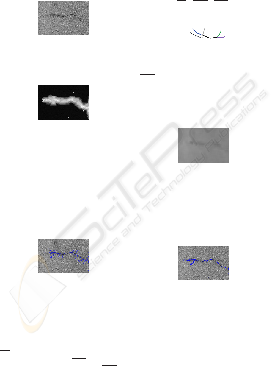
Figure 1: Initial image example (I(x, y, 1)) – The crack cor-

responds to a local low-contrasted heterogeneity.

the feature has been identiﬁed. Details identiﬁed with

a better precision have therefore a higher value (e.g.

Figure 2).

Figure 2: RGL image of Figure 1 (I

RGL

(x, y)) – The brighter

the pixels, the higher the precision of the detection.

The next step aims to thin the RGL image fea-

tures to obtain 1-pixel wide objects, and has been

adapted from our initial work to this road application.

It needed to be modiﬁed since, contrary to membrane

edges, cracks do no form closed regions: therefore,

we can either apply the watershed algorithm after con-

sidering the background of the RGL image as seeds

(i.e. pixels which value is 0 and which touch non− 0

value pixels), or by applying a gray-scale thinning al-

gorithm (Redding, 1996). For its simplicity and lower

computational time, the watershed approach has been

used in this study. The resulting image I

(e.g. Fig-

ure 3) points to the potential crack pixels (PCP).

Figure 3: Potential crack pixels from Figure 2 (I

displayed

in blue on the original image).

A last step has been added to validate I

and re-

duce the false detections: a PCP is validated if its

contrast is above a given threshold C

. To make the

measure more robust to the noise, instead of analyzing

each PCP independently, the contrast is averaged on

segments (a segment is a set of contiguous pixels hav-

ing at most two neighboring PCP, see Figure 4 for an

illustration of this vocabulary). The average contrast

seg

of a segment is the difference between the aver-

age gray-levelof the segment (GL

seg

), and the average

gray-level of the neighboring background (GL

Bkg

seg

= GL

Bkg

− GL

seg

. (3)

1 segment

Figure 4: A potential crack composed of 5 segments (each

having a different color).

Bkg

(e.g. Figure 5) is measured using a large ﬁlter

averaging the neighboring values of the background

(pixels not labeled as PCP). The ﬁlter kernel size did

not seem critical, but it should be large enough to re-

duce the inﬂuence of noise, and small enough to con-

sider the irregularities of the road: a 25 × 25 pixels

kernel was experimentally chosen.

Figure 5: Estimated background of Figure 1.

A segment is considered as targeting a crack if

seg

> C

(e.g. Figure 6). Measures have been real-

ized to set the main parameters of the algorithms, i.e.

the kernel size of the standard deviation ﬁlter and the

threshold C

; we identiﬁed that the best results were

obtained with a 5× 5 pixels kernel and C

= 50. We

will describe the analysis methodology, and we will

restrain the presentation of the inﬂuence of C

on the

results.

Figure 6: Final crack detected on Figure 1 (usingC

= 40).

4 ASSESSMENT

METHODOLOGY

To evaluate and compare the crack detection methods,

we had to choose: a/ the tested images, b/ how to de-

termine the "ground truth" segmentation or reference

segmentation and c/ the criteria in order to quantita-

tively evaluate the results.

VISAPP 2010 - International Conference on Computer Vision Theory and Applications

144

4.1 Images

The algorithms were evaluated on 3 sets of test im-

ages: on 14 synthetic crack images, on 10 real images,

and on 10 pre-processed real images. For synthetic

images, it is easy and reliable to give a ground truth

segmentation. For real images, estimate a "ground

truth" or a reference segmentation is more compli-

cated but the images are more realistic than the syn-

thetic images.

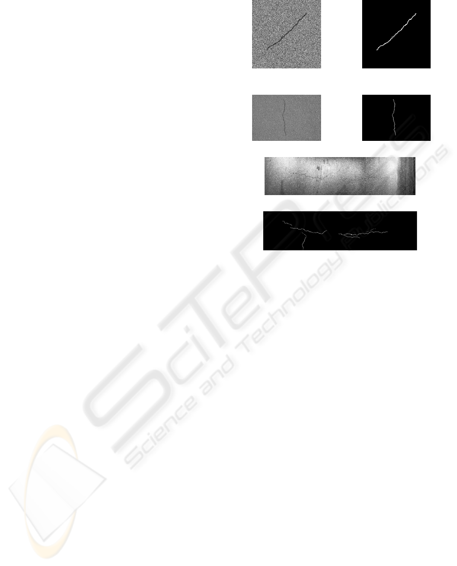
The 14 synthetic images were built using different

kinds of backgrounds: cracks were added on 8 im-

ages built with a random dot texture (sample S

), and

on 6 images of road containing no cracks, 2 of them

acquired with a static camera (sample S

), and 4 of

them dynamically acquired with a camera embedded

on a vehicle (sample S

). For the last four ones, con-

trolled lights were added. For all the 14 images, the

cracks were randomly added, with a random shape

and a random gray-level (Figure 7).

On the 10 real images, 4 were acquired using a

static camera and 6 using the dynamic system (Fig-

ure 7).

In the third set of test images, the 10 real images

were pre-processed using:

1. Threshold – In order to reduce the light halo in

some images (the last six ones presented in Fig-

ure 9), each pixel over a given threshold is re-

placed by the local average gray levels.

2. Smoothing – A mean ﬁlter of size 3×3 is applied.

3. Erosion – An erosion with a square structuring

element of size 3× 3 is applied.

4. Restoration – This last pre-processing tries to

combine the advantages of all the previous meth-

ods in three steps: histogram equalization, thresh-

olding (like Threshold), and erosion (like Ero-

sion).

4.2 Reference Segmentation

For real images, we brieﬂy explain how the manual

segmentation is validated. Four experts manually seg-

mented the images with the same tools and in the

same conditions. Then, the four segmentations were

merged, following these rules:

1. A pixel labeled as crack by almost two experts

was kept;

2. Every pixel near to a pixel kept by step 1 was also

kept.

The second rule is iterative and stops when no pixel is

added.

Synthetic image Ground truth

Real image + simulated

default

Ground truth

Real image manually segmented

Reference

Figure 7: Tested images.

Then, the result is dilated with a structuring ele-

ment of size 3× 3. Results of the manual segmenta-

tions are presented in Figure 9 (for more details, the

study of the reliability of these reference segmenta-

tions can be found in (Chambon et al., 2010)).

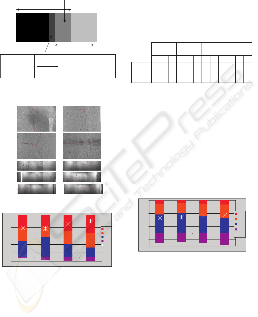
4.3 Quantitative Assessment

In Figure 8, the evaluation criteria are presented. They

are the most used in the literature, except "accepted"

pixels. In consequence, we have included accepted

pixels in the computation of the similarity coefﬁcient.

For estimating accepted pixels, a threshold is applied

on the distance between the detected pixel and the ref-

erence segmentation. This threshold is estimated us-

ing the mean distance between each of the four seg-

mentations used for establishing the reference.

The DICE values lie on the [0;1] interval, but to

simplify the visualization of the results, we display

DICE×100 in all ﬁgures and tables of section 5.

5 RESULTS AND DISCUSSION

5.1 Synthetic Images

Figure 10 compares results for the different meth-

ods with synthetic images. It shows that the multi-

resolution withC

= 50 is the best to identify most of

MULTI-RESOLUTION APPROACH FOR FINE STRUCTURE EXTRACTION - Application and Validation on Road

Images

145

Positives (P)

False

Positives

(FP)

Accepted

Corrects = True positives (TP)

Reference

Negatives

False

(FN)

Similarity

coefﬁcient or

Dice

similarity)

2TP

FN+TP+P

Ratio between good

detections and

non-detection

Figure 8: Evaluation criteria – Representation of the recov-

ery between an estimated segmentation (positives, P) and a

reference segmentation.

1 2

3 4

5 6

7 8

9 10

Figure 9: Manual ground truth segmentations.

-10

Acc

DICE

AFMM

= 30

= 40

= 50

MRDH

Figure 10: Summary of the algorithm performances on syn-

thetic images.

the edges, while the AFMM method is more adapted

to keep the proportion of FN low. By comparing

DICE values, the multi-resolution method appears to

be the most adapted.

Table 1 details the results for the different types

of images (samples S

to S

presented in section 4.1).

On fully synthetic images, both algorithms perform

very well. It appears that the images acquired with

the dynamic system are the most difﬁcult to process,

Table 1: Results on Synthetic Images – The 3 image cate-

gories are: S

, fully synthetic images, S

, background ac-

quired with a camera and S

, background acquired with

the dynamic system. Results in bold indicate best values

and it illustrates how the MRDH approach outperforms the

AFMM, in particular, with the most difﬁcult images (sam-

ple S

) where DICE is correct (greater than 50) whereas it

is very low with the other methods.

AFMM MRDH,

= 30

MRDH,

= 40

MRDH,

= 50

TP+Acc

87 46 15 68 41 30 86 53 43 91 66 59

FN 1.5 3.7 2.6 2.8 4.4 17 5.3 6.9 18 6.7 6.9 18

DICE

92 63 24 81 59 44 92 69 57 94 80 70

whatever the method used.

5.2 Real Images

Figure 11 displays the results obtained on the real im-

ages. We see that the amount of FN is higher than

with synthetic images, but we note that these values

are probably over-estimated,the human-referenceim-

ages tending to select only the major cracks. The

AFMM algorithm identiﬁed almost half of the cracks

selected by the human, and a bit more than half were

identiﬁed with the multi-resolution method. Consid-

ering the DICE measure, the multi-resolution tests

gave the best overall results; though, on camera ac-

quired images, DICE values can be considered as

equivalent for both methods.

-40

-20

100

Acc

DICE

AFMM

= 30 C

= 40 C

= 50

MRDH MRDH MRDH

Figure 11: Summary of the algorithm performances on real

images.

5.3 Real Pre-processed Images

Here, we compare the AFMM method with the

MRDH method (only the one with the more efﬁcient

parameter, i.e. C

= 50, is discussed here) when the

real images are pre-processed. In particular, we eval-

uate the inﬂuence of the 4 pre-processing described in

section 4.1.

Table 2 shows the DICE measures obtained. It

can be seen that the four pre-processings enhance the

overall performances.

VISAPP 2010 - International Conference on Computer Vision Theory and Applications

146

Table 2: DICE of pre-treated images: the three numbers

show the average values: with the 10 images (with the 4

images acquired in static way, with the 6 images acquired

in a dynamic manner).

AFMM MRDH, C

= 50

None 46 (49,44) 55 (52,57)

Threshold 64 (68,61) 55 (60,50)

Smoothing 66 (77,59) 52 (63,42)

Erosion 59 (58,60) 57 (64,51)

Restoration 52 (49,55) 57 (59,55)

When pre-processed with the threshold, smooth-

ing, erosion and restoration, the AFMM’s algorithm

is better, with the best results being obtained after a

smoothing. Also, smoothing and threshold have an

even more beneﬁcial effect when static images are

used.

According to the DICE measure, the perfor-

mances of MRDH applied after pre-treatment are

quite disparate. In fact, it illustrates how this new

method is globally quite robust against the acquisition

conditions. Images do not need to be pre-processed in

order to increase the performances and this is an im-

portant superiority compared to the AFMM method

which is highly dependent on the acquisition condi-

tions. Analyzed in details, we notice that for static

images, DICE values seem to be enhanced by each

pre-processing, while DICE values seem to decrease

for "dynamic" images.

6 CONCLUSIONS

A methodology for adapting a multi-resolution-based

segmentation to the ﬁeld of road crack detection has

been introduced. The experimental results demon-

strate the efﬁcient results obtained on 14 synthetic

images and 10 signiﬁcant real images. Moreover, it

shows how it outperforms a previous method based

on adapted ﬁltering, in particular with the most dif-

ﬁcult images acquired dynamically and that present

illumination defaults.

The next step of this work will be to validate this

work on more data (32 more images will be avail-

able soon). It has been shown that MRDH improves

the percentage of true detections (this percentage is

higher than with AFMM), but the AFMM presents

less false negatives. The next improvement will be

to reduce this phenomenon by introducing more con-

straints on the ﬁnal step, like for example, an active

contour constraint instead of using only the constraint

on the contrast.

REFERENCES

Bray, J., Verma, B., Li, X., and He, W. (2006). A neural

nework based technique for automatic classiﬁcation

of road cracks. In International Joint Conference on

Neural Networks, pages 907–912.

Chambon, S., Gourraud, C., Moliard, J.-M., and Nicolle, P.

(2010). Road crack extraction with adapted ﬁltering

and markov model-based segmentation. In VISAPP.

Coudray, N., Buessler, J.-L., Kihl, H., and Urban, J.-P.

(2007). Tem images of membranes: a multiresolu-

tion edge-detection approach for watershed segmenta-

tion. In Physics in Signal and Image Processing (PSIP

2007).

Elbehiery, H., Hefnawy, A., and Elewa, M. (2005). Sur-

face defects detection for ceramic tiles using image

processing and morphological techniques. Proceed-

ings of World Academy of Science, Engineering and

Technology (PWASET), 5:158–162.

Frangi, A. F., Niessen, W. J., Vincken, K. L., and Viergever,

M. A. (1998). Muliscale vessel enhancement ﬁltering.

In MICCAI, pages 130–137.

Geman, D. and Jedynak, B. (1996). An active testing model

for tracking roads in satellite images. IEEE Pattern

Analysis and Machine Intelligence, 18(1):1–14.

Iyer, S. and Sinha, S. (2005). A robust approach for auto-

matic detection and segmentation of cracks in under-

ground pipeline images. Image and Vision Computing,

23(10):921–933.

Koutsopoulos, H. and Downey, A. (1993). Primitive-based

classiﬁcation of pavement cracking images. ASCE,

Journal of Transportation Engineering, 119(3):402–

418.

Redding, N. (1996). The autoscaling of oblique ionograms.

Technical report, Defence science and technology or-

ganization canberra.

Schmidt, B. (2003). Automated pavement cracking assess-

ment equipment – state of the art. Technical Report

320, Surface Characteristics Technical Committee of

the World Road Association (PIARC).

Subirats, P., Fabre, O., Dumoulin, J., Legeay, V., and Barba,

D. (2006). Automation of pavement surface crack de-

tection with a matched ﬁltering to deﬁne the mother

wavelet function used. In European Signal Process-

ing Conference.

Tanaka, N. and Uematsu, K. (1998). A crack detection

method in road surface images using morphology.

In Workshop on Machine Vision Applications, pages

154–157.

MULTI-RESOLUTION APPROACH FOR FINE STRUCTURE EXTRACTION - Application and Validation on Road

Images

147