
SWEEPING BASED CONTROLLABLE SURFACE BLENDING
L. H. You
1
, H. Ugail
2
, B. P. Tang
3
, X. Y. You
4
and Jian J. Zhang
1
1
National Centre for Computer Animation, Bournemouth University, U.K.
2
School of Computing, Informatics and Media, University of Bradford, U.K.
3
College of Mechanical Engineering, Chongqing University, Chongqing City, China
4
Faculty of Engineering and Computing, Coventry University, U.K.
Keywords: Surface Blending, Controllable Shapes, Vector-valued Fourth Order Ordinary Differential Equation.
Abstract: In this paper, we propose a novel sweeping surface based blending method. A generator defined by the
solution of a vector-valued fourth order ordinary differential equation is swept along the two trimlines,
which meets the boundary tangent constraints of the primary surfaces at the trimlines. The blending surface
generated therefore satisfies both the positional and tangential continuity constraints at the interfaces
between the primary surfaces and the blending surface. Since the vector-valued shape control parameters are
embedded in the blending surface, its shape can be effectively controlled and manipulated by adjusting
these vector-valued shape control parameters. Several surface blending examples are given to demonstrate
the applications of the proposed method.
1 INTRODUCTION
In computer-aided design and geometric modeling,
often it requires to smoothly connect two separate
surfaces together. This operation is called surface
blending. The surfaces to be connected are called the
primary surfaces. The surface which forms a smooth
transition between the primary surfaces is called a
blending surface. The interfaces between the
primary surfaces and the blending surface are called
trimlins. The geometric properties at the trimlines
form the boundary conditions, which need to be
satisfied when a blending surface is generated.
Surface blending has been a research topic for
decades especially in computer-aided design.
Recently, it has found its way to character modeling
in 3D animation. Several surface blending methods
have been proposed in the existing literature.
The rolling-ball method is the most popular. It
was pioneered by Rossignac and Requicha (1984).
According to different surface representations, the
rolling-ball blending method can be classified into
those of implicit surfaces and parametric surfaces.
Lukács (1998) discussed how to blend implicit
surfaces using the rolling-ball method. Kós et al.
(2000) investigated how to recover constant radius
rolling ball blends used in reverse engineering. For
the rolling-ball blending of parametric surfaces, two
different blends can be identified depending on
whether the radius of the rolling ball varies or not.
One is the constant-radius rolling-ball blend method,
and the other is variable-radius rolling-ball blend
method. The constant-radius rolling-ball blend
method is studied by Choi and Ju (1989), Harada et
al. (1990), Sanglikar et al. (1990), Ying et al. (1991),
Barnhill et al. (1993), and Farouki and Sverrisson
(1996). The variable-radius rolling-ball blend
method is addressed by Harada et al. (1991), Chuang
et al. (1995), Chuang and Hwang (1997), Chuang
and Lien (1998), and Hartmann (2000).
Cyclides are also useful in some simple blending
tasks such as a cylinder obliquely meeting a plane.
In general, implicit quartic equations or parametric
representations in the form of trigonometrical
parameterisation or rational biquadratic Bézier
equations are used to describe cyclides. Cyclides
were investigated by Allen and Dutta (1997a,
1997b), and Shene (1998).
Partial differential equations (PDEs) based
surface blending was pioneered by Bloor and Wilson
(1989). In the work, a biharmonic-like fourth order
PDE with one vector-valued parameter was used to
solve blending problems. The perturbation method
developed by Bloor and Wilson (2000) is suitable
for solving more complicated surface blending
problems than their previously proposed analytical
solution. In order to improve the capability of PDE
based surface blending, numerical methods were
introduced to solve partial differential equations and
78
H. You L., Ugail H., P. Tang B., Y. You X. and J. Zhang J. (2010).
SWEEPING BASED CONTROLLABLE SURFACE BLENDING.
In Proceedings of the International Conference on Computer Graphics Theory and Applications, pages 78-83
DOI: 10.5220/0002823000780083
Copyright
c
SciTePress

created blending surfaces. Following their analytical
work, Bloor and Wilson (1990) developed a
collocation method based on B-spline representation
of blending surfaces. Finite difference method was
proposed by Cheng et al. (1990) to solve a vector-
valued fourth order partial differential equation for
generation of blending surfaces between two
cylinders and between a cone and a cylinder. At the
same year, a B-spline finite element method was
presented by Brown et al. (1990). Later on, a
boundary penalty finite element method was
investigated by Li (1998, 1999) and Li and Chang
(1999). By studying an efficient semi-analytical and
semi-numerical method, You et al. (2004a, 2004b)
used a vector-valued fourth order partial differential
equation to generate blending surfaces with
tangential continuity and a vector-valued sixth order
partial differential equation to create blending
surfaces with curvature continuity.
In contrast to the applications of partial
differential equations in geometric modelling, little
work exists where ordinary differential equations
were used for geometric modelling and computer
animation. Surface creation and manipulation with
time-independent ordinary differential equations was
investigated by You et al. (2007). By introducing a
time variable and considering the dynamic effect,
time-dependent ordinary differential equations were
applied in animating skin shapes in character
animation (You et al. 2008).
Up to now, we have not found any publications
investigating ordinary differential equation based
surface blending. This paper will address this issue.
It uses the solutions to a vector-valued fourth order
ordinary differential equation together with the
boundary conditions to create a blending surface;
and to control the shape of the blending surface
through the manipulation of the shape control
parameters involved in the equation.
2 MATHEMATICAL MODEL AND
SOLUTION
Surface blending with tangential continuity is most
frequently met in computer-aided design and
geometric modelling. In this paper, we concentrate
on such surface blending tasks.
The boundary conditions for surface blending
with tangential continuity consist of the positional
and tangential information of the primary surfaces at
the trimlines, i.e., boundary curves and boundary
tangents. They can be represented with the equation
below.
)( )( 1
)( )( 0
11
00
v
u
vu
v
u
vu
C
X
CX
C
X
CX
(1)
where subscript 0 indicates the boundary
0u and
subscript 1 indicates the boundary
1u , those
without an overbar denote boundary curves, and
those with an overbar stand for boundary tangents.
In equation (1), all the vector-valued functions
)(
0
vC , )(
0
vC , )(
1
vC and )(
1
vC have three
components. Taking the vector-valued
function
)(
0
vC to be an example, the three
components can be written as
)(
0
vC
x
, )(
0
vC
y
and
)(
0
vC
z
and ))(),(),(()(
0000
vCvCvCv
zyx
C .
A blending surface can be created by sweeping a
generator along two trimlines and satisfying the
tangential continuity at the trimlines. If the
mathematical representation of a blending surface is
),( vuS , the mathematical representation of the
generator at the position
i
v is ),()(
i
vuu SG .
In order to control the shape of a blending
surface, we must deform the generator. Through the
following fourth order ordinary differential equation,
the generator is related to vector-valued shape
control parameters which will be used to manipulate
the generator.
0)(
)()(
2
2
4
4
u
du
ud
du
ud
dG
G
c
G
b (2)
where
b , c and d are vector-valued shape control
parameters, and
)(uG has three components
)(uG
x
,
)(uG
y
and )(uG
z
.
The analytical solution of equation (2) can be
taken to be
ru
eu )(G
(3)
Substituting equation (3) into (2), the ordinary
differential equation is changed into an algebra
equation below
0
24
dcb rr (4)
Depending on combinations of the vector-valued
shape control parameters, equation (4) has different
solutions. Here, we only consider the situation of
bdc 4
2
and 0/
bc .
For this situation, the roots of equation (4) are
14,3,2,1
qr
(5)
where
SWEEPING BASED CONTROLLABLE SURFACE BLENDING
79
)2/(
1
bcq
(6)
With the roots given in equation (5), the solution
of equation (2) is
uquququq
ueeueeu
1111
4321
)(
ccccG (7)
where
4321
,,, cccc
are unknown constants which will
be determined below.
The unknown constants in equation (7) can be
determined by substituting it into boundary
conditions (1).
With the obtained solution, we can generate
blending surfaces constrained by boundary
conditions (1).
3 SHAPE CONTROL OF
BLENDING SURFACES
In this section, we investigate how the vector-valued
shape control parameters are used to control the
shape of blending surfaces through a surface
blending example below.
This blending task is to find a transition surface
which smoothly connects an open surface and a
cylinder together. The boundary conditions for this
blending task can be written as
2
10
43
210
0
0 sin
0 cos1
0
00
h
u
z
z
u
y
v ry
u
x
v r xu
h
u
z
hz
u
y
v ddy
u
x
edvdd xu
v
(8)
where
i
d (i=0,1,2,3,4),
i
h (i=0,1,2), and
r
are
known constants.
For the blending surface given in Figure 1,
5001.0
0
d , 1584.0
1
d ,
4
2
1002.1
d , 5.1
3
d ,
4775.0
4
d
, 0.2h ,
0.2
21
hh
, and 0.1
r .
By solving Eq. (2) subjected to boundary
conditions (8), we obtained the analytical solution.
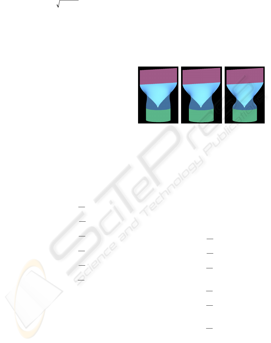
Initially, we set the vector-valued shape control
parameters
1b , and 3
c . The blending surface
indicated in Figure 1a was created. Then, we
changed the vector-valued shape control parameter
c to -15, the blending surface depicted in Figure 1b
was generated. Finally, we further changed the shape
control parameter to -30, the blending surface in
Figure 1b was changed into that in Figure 1c.
Comparing these figures, we can conclude that the
vector-valued shape control parameters can be used
to change the shape of a blending surface but still
maintain the original boundary conditions of the
blending task.
a b c
Figure 1: Different shapes of the blending surface created
by different vector-valued shape control parameters.
4 APPLICATION EXAMPLES
In this section, we give a number of examples to
demonstrate the applications of the proposed method
in surface blending.
The first example is to generate a blending
surface between the frustum of an irregular conical
surface and an elliptic cylinder. The boundary
conditions for this blending task are
h
u
z
uhvaz z
u
y
v b y
h
u
x
αuhvαax xu
h
u
z
uh z
vvR
u
y
v vRu y
vR
u
x
v Ru xu
cos
coscossin
0 sin
sin
sincoscos1
sin sin
cos cos0
1
0110
1
0110
000
0
0
(9)
where
R
,
R
,
0
u ,
01
u ,
0
h ,
0
h
,
1
h ,
1
h
,
0
x ,
0
z , a ,
b , and
are known constants.
Using the same method, we obtained the
analytical solution of equation (2).
GRAPP 2010 - International Conference on Computer Graphics Theory and Applications
80
Taking the geometric parameters in the above
equation to be:
2.1
RR , 2
00
hh , 3.0
0
u ,
1
010
ux , 8.0a , 6.0
b ,
o
40
, 5.1
1
h ,
2
1
h , and 9.1
0
z , and setting the vector-valued
parameters
a and c to 1, and b to -5, the blending
surface created from the analytical solution is shown
in Figure 2.
Figure 2: Blending between the frustum of an irregular
conical surface and an elliptic cylinder.
The second example is to blend an ellipsoid to an
elliptic paraboloid. The boundary conditions for this
blending task are
13
3
1323
1
2
12
1
1
11
01
3
2
0103
2
02
1
01
sin cos
sincos ssin
coscos cossin 1u
sin sin
cos cos 0
uh
u
x
uhhx
vub
u
x
invubx
vua
u
x
vuax
uh
u
x
uhhx
vd
u
x
vdux
vc
u
x
v cuxu
(10)
where
c , d , d
,
0
h
,
1
h
,
1
h
, a , a
, b , b
,
2
h
,
3
h
,
3
h
,
0
u , and
1
u are known constants.
Using the same treatment, we obtained the
analytical solution of this blending task which was
used to produce the blending surface shown in
Figure 3.
Figure 3: Blending between an ellipsoid and an elliptic
paraboloid.
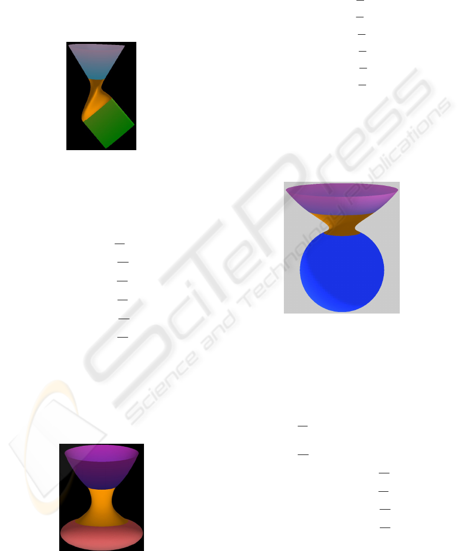
The third example is to investigate the blending
between an elliptic paraboloid and a sphere. The
boundary conditions for this blending task have the
form of
sin cos
sincos sinsin
coscos cossin 1
2
sin sin
cos os 0
0101
0101
0101
01
2
010
0
0
uR
u
z
uRz
vuR
u
y
vuRy
vuR
u
x
vuRxu
uh
u
z
uhhz
vb
u
y
v buy
va
u
x
vcauxu
(11)
where
a , a
, b , b
,
0
h ,
1
h ,
1
h
,
R
,
R
,
0
u , and
01
u
are known constants.
With the method discussed above, the blending
surface was obtained from equation (2) and the
above boundary conditions. It was depicted in
Figure 4.
Figure 4: Blending between an elliptic paraboloid and a
sphere.
The fourth example is to blend an open surface
to a plane at a specified pedal-like curve. The
boundary conditions for this surface blending take
the form of
0
cos )cos(cos
sin )sin(sin 1
e
cos
cos)cosh(
sin
sin)sinh( 0
3
13
2
82
1
81
2.0
3
0.2
03
5
2
4762
5
1
43211
u
x
hx
va
u
x
vabvax
va
u
x
vabvaxu
e
u
x
hx
va
u
x
v avaax
va
u
x
vaavaaxu
(12)
where
i
a (i=1,2,…, 8),
0
h , and
1
h are known
constants.
SWEEPING BASED CONTROLLABLE SURFACE BLENDING
81
Using the analytical solution obtained from
equation (2) and the above boundary conditions, the
blending surface was created and indicated in Figure
5.
Figure 5: Blending between an open surface and a plane at
a specified pedal-like curve.
The fifth example is to generate a blending
surface between a circular cylinder and an elliptic
hyperboloid of two sheets. The boundary conditions
for this blending task are given below.
1sinh cosh1
sin1cosh sin1sinh
cos1cosh cos1sinh
1
0 sin
0 cos
0
11
00
h
u
z
hz
vb
u
y
vby
va
u
x
vax
u
h
u
z
hz
u
y
vR y
u
x
vRx
u
(13)
where
R
, a , a
, b , b
,
0
h ,
0
h
,
1
h and
1
h
are
known constants.
The blending surface produced from the solution
to equation (2) subjected to the above boundary
conditions was given in Figure 6.
Figure 6: Blending between a circular cylinder and an
elliptic hyperboloid of two sheets.
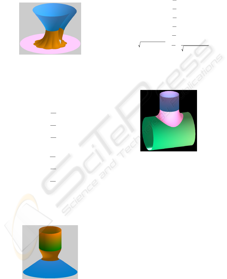
The last example is to smoothly connect two
intersecting cylinders together. The boundary
conditions for this blending task can be written as
vlsr
vt
u
z
vlsrz
vt
u
y
vlsy
vt
u
x
vlsxu
h
u
z
hz
u
y
vsy
u
x
vsxu
2
2
1
2
2
2
2
1
2
1
1
10
cos
cos
cos=
sin sin
cos cos 1
=
0 sin
0 cos 0
(14)
where
s
,
0
h
,
1
h
,
1
l
, t , and
r
are known constants.
Using the same treatment, analytical solution of
equation (2) under boundary conditions (14) was
obtained which was used to generate the blending
surface indicated in Figure 7.
Figure 7: Blending between two intersecting cylinders.
5 CONCLUSIONS
With our new surface blending method, a sweeping
surface is generated along two trimlines. The key
task is to ensure that this sweeping surface satisfies
the tangential continuity constraints at the trimlines.
The shape of the generator is controlled by the
vector-valued shape parameters associated with the
fourth order ordinary differential equation. This
makes the blending surfaces controllable and
applicable for different conditions and applications.
The validity of the proposed method is demonstrated
with application examples given in this paper.
Since our proposed blending method is based on
the closed form solution to a vector-valued fourth
order ordinary differential equation, it is simple and
efficient in creating blending surfaces. We intend to
implement it into a user-friendly interface for
interactive shape manipulation of blending surfaces
and apply this method to tackle more surface blen-
GRAPP 2010 - International Conference on Computer Graphics Theory and Applications
82

ding problems in our future work.
REFERENCES
Rossignac, J.R., Requicha, A.A.G., 1984. Constant-radius
blending in solid modeling, Computers in Mechanical
Engineering, 65-73.
Lukács, G., 1998. Differential geometry of
1
G variable
radius rolling ball blend surfaces, Computer Aided
Geometric Design 15, 585-613.
Kós, G., Martin, R.R., Várady, T., 2000. Methods to
recover constant radius rolling ball blends in reverse
engineering, Computer Aided Geometric Design 17,
127-160.
Barnhill, R.E., Farin, G.E., Chen, Q., 1993. Constant-
radius blending of parametric surfaces, Computing
Supple 8, 1-20.
Choi, B.K., Ju, S.Y., 1989. Constant-radius blending in
surface modeling, Computer Aided Design 21(4), 213-
220.
Harada, T., Toriya, H., Chiyokura, H., 1990. An enhanced
rounding operation between curved surfaces in solid
modelling, In Proceedings of CG International '90.
Computer Graphics Around the World, Singapore, 25-
29 June, pp. 563-588.
Sanglikar, M.A., Koparkar, P., Joshi, V.N., 1990.
Modelling rolling ball blends for computer aided
geometric design, Computer Aided Geometric Design
7, 399-414.
D.-N. Ying, E.-J. Wang and K. Xue. Blending in solid
modelling. Proceedings of First International
Conference on Computational Graphics and
Visualization Techniques, Sesimbra, Portugal, 16-20
Sept. 1991, Vol. 2, pp. 239-247.
Farouki, R.A.M.T., Sverrisson, R., 1996. Approximation
of rolling-ball blends for free-form parametric
surfaces, Computer Aided Design 28(11), 871-878.
Allen, S., Dutta, D., 1997a. Cyclides in pure blending I,
Computer Aided Geometric Design 14, 51-75.
Allen, S., Dutta, D., 1997b. Supercyclides and blending,
Computer Aided Geometric Design 14, 637-651.
Shene, C.-K., 1998. Blending two cones with Dupin
cyclides, Computer Aided Geometric Design 15, 643-
673.
Bloor, M.I.G., Wilson, M.J., 1989. Generating blend
surfaces using partial differential equations,
Computer-Aided Design 21(3), 165-171.
Bloor, M.I.G., Wilson, M.J., 1990. Representing PDE
surfaces in terms of B-splines, Computer-Aided
Design 22(6), 324-331.
Cheng, S.Y., Bloor, M.I.G., Saia, A., Wilson, M.J., 1990.
Blending between quadric surfaces using partial
differential equations, in Ravani, B. (Ed.), Advances in
Design Automation, vol. 1, Computer and
Computational Design, ASME, 257-263.
Brown, J.M., Bloor, M.I.G., Susan, M., Wilson, M.J.,
1990. Generation and modification of non-uniform B-
spline surface approximations to PDE surfaces using
the finite element method, in Ravani, B. (Ed.),
Advances in Design Automation, Vol. 1, Computer
Aided and Computational Design, ASME, 265-272.
Li, Z.C., 1998. Boundary penalty finite element methods
for blending surfaces, I. Basic theory, Journal of
Computational Mathematics 16, 457-480.
Li, Z.C., 1999. Boundary penalty finite element methods
for blending surfaces, II. Biharmonic equations,
Journal of Computational and Applied Mathematics
110, 155-176.
Li, Z.C., Chang, C.-S., 1999. Boundary penalty finite
element methods for blending surfaces, III,
Superconvergence and stability and examples, Journal
of Computational and Applied Mathematics 110, 241-
270.
Bloor M.I.G., Wilson, M.J., 2000. Generating blend
surfaces using a perturbation method, Mathematical
and Computer Modelling 31(1), 1-13.
You, L.H., Zhang J.J., Comninos, P., 2004a. Blending
surface generation using a fast and accurate analytical
solution of a fourth order PDE with three shape
control parameters, The Visual Computer20, 199-214.
You, L.H., Comninos, P., Zhang, J.J., 2004b. PDE
blending surfaces with
2
C continuity, Computers &
Graphics28(6), 895-906.
You, L.H. Yang, X.S., Pachulski, M. and Zhang, J.J.,
2007. Boundary Constrained Swept Surfaces for
Modelling and Animation, EUROGRAPHICS 2007
and Computer Graphics Forum 26(3), 313-322.
You, L.H., Yang, X.S., Zhang, J.J., 2008. Dynamic skin
deformation with characteristic curves, Computer
Animation and Virtual Worlds 19(3-4), 433-444.
SWEEPING BASED CONTROLLABLE SURFACE BLENDING
83
