
DYNAMIC GLOBAL OPTIMIZATION FRAMEWORK FOR
REAL-TIME TRACKING
João F. Henriques, Rui Caseiro and Jorge Batista
Institute of Systems and Robotics, Department of Electrical and Computer Engineering
University of Coimbra, Portugal
Keywords:
Visual surveillance, Tracking, real-time, Dynamic Hungarian algorithm, Region covariance matrices.
Abstract:
Tracking is a crucial task in the context of visual surveillance. There are roughly three classes of trackers: the
classical greedy algorithms (based on sequential modeling of targets, such as particle filters), Multiple Hy-
pothesis Tracking (MHT) and its variants, and global optimizers (based on optimal matching algorithms from
linear programming). We point out the shortcomings of all approaches, and set out to solve the only gaping
deficiency of global optimization trackers, which is their inability to work with streamed video, in continual
operation. We present an extension to the new Dynamic Hungarian Algorithm that achieves this effect, and
show tracking results in such different conditions as the tracking of humans and vehicles, in different scenes,
using the same set of parameters for our tracker.
1 INTRODUCTION
The past few years have seen an increased interest in
the development of automatic surveillance systems.
Many approaches are based exclusively on the inter-
pretation of color camera images (as opposed to, for
example, multi-sensor networks), since it would al-
low relatively easy integration with existing CCTV
camera networks. Security and monitoring applica-
tions require that a system is capable of (a) detect-
ing people, (b) tracking them while maintaining their
true identities over difficult situations such as occlu-
sion and appearance changes, and (c) identifying and
reacting to their behavior. The focus of this work is
the second task.
Many approaches have been proposed since au-
tomatic tracking became feasible, but only recently
has a significant breakthrough been made: the use of
global optimization methods.
Trackers of this type have an enormous advantage
over classical trackers, since they rely on the use of
global information. Trackers based on Kalman filters,
particle filters (Palaio and Batista, 2008; Okuma et al.,
2004) and other ad-hoc greedy algorithms (Betke
et al., 2007; Shafique and Shah, 2005) are all exam-
ples of classical trackers. Classical tracking systems
are greedy, in that they’re limited to information about
the current frame, and a summary of the information
from previous frames (i.e., the filters’ states, a list of
tracked objects, etc). This often leads to trapping in
local minima of the functions they try to optimize, and
drifting when faced with ambiguities that can’t be re-
solved immediately. The popular Multiple Hypoth-
esis Tracker (MHT) (Reid, 1979) improves on this,
and can be seen as a transitional step between greedy
methods and global optimization. However, the com-
binatorial explosion from all the different possibilities
under consideration limits its window of operation to
no more than a few frames. The global methods we
refer to, based on the Hungarian algorithm (Stauffer,
2003; Taj et al., 2007), enjoy a much smaller compu-
tational complexity, since they take advantage of the
sub-structure of the matching problem; their worst-
case running time is O(n
3
), where n is the number
of detections over all frames under consideration (in-
stead of exponential). The earliest uses of the Hungar-
ian algorithm in tracking applications were the match-
ing of objects from different cameras with disjoint
views (Huang and Russell, 1997), where it remains a
popular algorithm (Javed et al., 2003), but since then
it has been generalized for tracking within a single
camera.
One way to reduce n substantially, improving
running times by an order of magnitude, is pre-
computing tracklets using a conservative strategy (de-
scribed in Section 2.1). Evidence of this sort of rea-
soning can be found in several other works, under dif-
ferent names. Kanade et al. (Li et al., 2008) uses a
track compiler to produce track segments, associated
later by a track linker (these terms correspond, respec-
207
Henriques J., Caseiro R. and Batista J. (2010).
DYNAMIC GLOBAL OPTIMIZATION FRAMEWORK FOR REAL-TIME TRACKING.
In Proceedings of the International Conference on Computer Vision Theory and Applications, pages 207-215
DOI: 10.5220/0002823502070215
Copyright
c
SciTePress

tively, to our conservative association, tracklets and
optimal association). Stauffer (Stauffer, 2003) refers
to the later as track stitching. Both Stauffer and Neva-
tia (Huang et al., 2008) refer to the track segments as
tracklets.
An inherent issue of global optimization is easy to
understand: in a realistic scenario, we obviously don’t
have access to the whole video to analize it globally;
instead, a continuous video stream is received over
time, and we wish to obtain tracking results as imme-
diately as possible. To this date, this promising class
of methods hasn’t been able to make the leap from
global analysis of a single video segment to analy-
sis of continuous video streams. Our work intends to
bridge this gap, through the method outlined in Sec-
tion 4.
This paper is organized as follows. Section 2 de-
scribes the tracking framework based on a probabilis-
tic formulation of the problem, which is then solved
by the Hungarian Algorithm. Section 3 showcases
the appearance descriptor of our choice, the Region
Covariance Matrix (RCM). Section 4 presents the ex-
tension of the Dynamic Hungarian Algorithm to deal
with a sliding window, enabling its use in continuous,
streamed video, as opposed to small video segments
as has been the case in previous work. Finally, Sec-
tions 5 and 6 show, respectively, the experimental re-
sults and our conclusions.
2 TRACKING METHODOLOGY
Our tracking method starts with a stripped-down im-
plementation of the hierarchical tracker proposed by
Nevatia et al. (Huang et al., 2008). Their work fol-
lows the recent trend of computing association scores
between all pairs of detections and using the Hun-
garian algorithm to create a matching between them
1
, thus obtaining a set of tracks, in a way that opti-
mizes the association scores. They computed the as-
sociations progressively, through a hierarchy of low,
middle and high-level association schemes; the basic
framework for our tracker is adapted from theirs, and
will be described in this section.
2.1 Conservative Association
Recall that the main objective is to associate (match)
each detection to another one, optimizing some asso-
ciation criteria. In a typical scene, there’s a good num-
ber of associations that are straightforward to com-
pute. For example, a person walking down a corridor
1
In the tracking context, a matching indicates, for each
detection, which one comes next.
alone without any occlusion will yield a set of detec-
tions with high association scores, and no other detec-
tions should have equally high scores towards those
detections. In such cases matching is easily computed
and is unambiguous, by a process we call conserva-
tive association. This turns out to be an efficient op-
timization, relieving the Hungarian algorithm of this
duty (the algorithm’s running time is O(n
3
), with n
the number of detections).
2.1.1 Conservative Strategy
We denote r
i
as a detection response, which may con-
tain characteristics such as position, frame index, and
appearance properties. Instead of arbitrary scores, it
makes sense to maximize association probabilities, so
these will be used throughout the text. The aim of
this first take on matching is to consider matches that
have a high association probability (higher than an
arbitrary threshold θ
1
), but only if there is no other
conflicting match; that is, all other matches involving
these two detections have lower probabilities (by at
least θ
2
). This is defined in (1), where P
link
(r
i
|r
j
) is
the association probability between detections r
i
and
r
j
.
P
link
(r
i
|r
j
) > θ
1
min
P
link
(r
i
|r
j
) − P
link
(r
k
|r
j
),
P
link
(r
i
|r
j
) − P
link
(r
i
|r
k
)
> θ
2
,
∀r
k
∈ R −
r
i
,r
j
(1)
2.1.2 Association Probabilities
The association probabilities can be computed
through (2), which is simply the joint probability
of three probabilities of identity, called affinities.
A
δ
(r
i
|r
j
), δ ∈
{
p,s,a
}
are position, size and appear-
ance affinities (described in the next paragraph), and
t
k
is the frame index of the occurrence of detection r
k
.
Note that the only way for an association probability
to be non-zero is for the second detection to appear
exactly one frame after the first. This is part of the
conservative strategy, as occlusions (i.e., frame gaps
between detections) are not resolved at this stage.
P
link
(r
i
|r
j
) =
A
p
(r
i
|r
j
)A
s
(r
i
|r
j
)A
a
(r
i
|r
j
), if t
j
−t
i
= 1
0, otherwise
(2)
The position difference between two detections is
modeled through a two-dimensional Gaussian distri-
bution so the position affinity can be obtained from
the positions of two detections, p
i
and p
j
, as G(p
i
−
VISAPP 2010 - International Conference on Computer Vision Theory and Applications
208

p
j
; 0, Σ) (a Gaussian with zero mean and covariance
matrix obtained from sample data). Likewise for the
size affinity and appearance affinity. The later is ob-
tained from the dissimilarity metric described in Sec-
tion 3, this time using a single-dimensional Gaussian
distribution.
The result of this stage is a set of early matches,
that by no means have to include all of the detec-
tions. They represent a disjointed set of track seg-
ments, called tracklets. These tracklets can be further
associated by the Hungarian algorithm as described in
Section 2.2.
2.2 Optimal Association
As was stated before, the Hungarian algorithm (Kuhn,
1955) computes an optimal matching of detections.
Specifically, we can assign each possible match
(T
i
,T
j
) a cost c
i j
, through a cost matrix C; the al-
gorithm will compute the set of independent matches
that minimizes the sum of all costs.
2.2.1 MAP Formulation
In (Huang et al., 2008), the objectives of tracking are
stated as the MAP problem (3), where S is a set of
tracks, S
∗
is the optimal set of tracks, and T is the set
of all tracklets, through direct application of Bayes’
theorem.
S
∗
= arg max
S
P(S |T ) = arg max
S
P(T |S )P(S )
= arg max
S
∏
T
i
∈T
P(T
i
|S )
∏
S
k
∈S
P(S
k
) (3)
The conditional probability of a tracklet given the
set S depends on its inclusion in the solution, and is
modeled by a Bernoulli distribution from the hit rate
β of the detector and the number of elements |T
i
| in
the tracklet (4).
P(T
i
|S ) =
(
P
+
(T
i
) = β
|T
i
|
, if ∃S
k
∈ S , T
i
∈ S
k
P
−
(T
i
) = (1 − β)
|T
i
|
, otherwise
(4)
Finally, the prior probability of an association of
tracklets S
k
is a Markov Chain with initialization and
termination probabilities P
init
and P
term
, and a series
of link probabilities covering all the tracklets in the
sequence (5).
P(S
k
) = P
init
(T
i
0
)P
link
(T
i
0
|T
i
1
) (. . .)
P
link
(T
i
(n
k
−1)
|T
i
(n
k
)
)P
term
(T
i
(n
k
)
) (5)
The link probabilities, similarly to Section 2.1.2,
are given by the joint probabilities of motion (A
m
),
temporal (A
t
) and appearance (A
a
) affinities, as shown
in (6). Due to space limitations we won’t get into
much details about the motion and temporal compo-
nents, as this is explained thoroughly in (Huang et al.,
2008). The temporal component is modeled through
a Bernoulli distribution according to the time gap be-
tween two tracklets. The motion affinity is obtained
by projection through the time gap, assuming a con-
stant velocity model obtained with a Kalman filter,
and finally the projected positions are modeled with
Gaussians (similarly to the position affinity described
in Section 2.1.2). The appearance component is cal-
culated in the same way as in Section 2.1.2.
P
link
(T
i
|T
j
) = A
m
(T
i
|T
j
)A
t
(T
i
|T
j
)A
a
(T
i
|T
j
) (6)
2.2.2 Cost Matrix Definition
The above formulation can be decomposed into the
elements of a cost matrix (7), in such a way that the
optimal matching corresponds to the solution to the
MAP problem.
C =
c
11
c
12
··· c
1n
f
1
∞ ··· ∞
c
21
c
22
··· c
2n
∞ f
2
··· ∞
.
.
.
.
.
.
.
.
.
.
.
.
.
.
.
.
.
.
.
.
.
.
.
.
c
n1
c
c2
··· c
nn
∞ ∞ ··· f
n
i
1
∞ ··· ∞ 0 0 ·· · 0
∞ i
2
··· ∞ 0 0 ·· · 0
.
.
.
.
.
.
.
.
.
.
.
.
.
.
.
.
.
.
.
.
.
.
.
.
∞ ∞ · · · i
n
0 0 ·· · 0
(7)
The off-diagonal elements of the upper-left block
represent regular tracklet-to-tracklet matches. A se-
quence of matches of this nature will constitute a
track. A match to a diagonal element represents a
false alarm: tracklets in this situation are left out of
the final set of tracks and ignored entirely. Matches to
the diagonal elements of the upper-right block termi-
nate tracks, while matches to the diagonal elements of
the bottom-left block initiate tracks. The bottom-right
block is unused and any match occurring here incurs
no penalty.
c
i j
=
(
-log P
−
(T
i
), if i = j
-log
h
p
P
+
(T
i
)P
link
(T
i
,T
j
)
p
P
+
(T
j
)
i
, otherwise
i
k
= −log
h
P
init
(T
k
)
p
P
+
(T
k
)
i
f
k
= −log
h
P
term
(T
k
)
p
P
−
(T
k
)
i
DYNAMIC GLOBAL OPTIMIZATION FRAMEWORK FOR REAL-TIME TRACKING
209

2.2.3 Optimal Matching and Obtaining the
Objects’ Tracks
The Hungarian algorithm (Kuhn, 1955) is well-
known and described extensively in the literature
(Ahuja, 2008). It finds the optimal matching M
∗
given
the cost matrix C, in the form shown in (8).
M
∗
=
(T
i
,T
j
)|i, j ∈ 1, . . . , n
(8)
For this result to be meaningful in the tracking
context, we need to obtain a set of tracks, each one
composed of a sequence of tracklets. This can be done
by resorting to a connected components algorithm.
Given a 2n×2n matrix C, we’re only interested in
the first n elements of the matching M
∗
, which repre-
sent matches between tracklets, and false alarms (in
the form (T
i
,T
i
)). An n × n adjacency matrix A
∗
can
be constructed as described in (9).
A
∗
=
a
i j
, a
i j
=
(
1, if (T
i
,T
j
) ∈ M
∗
0, otherwise
(9)
Finding the connected components in the graph
represented by A
∗
, one gets a set of independent tracks
S
∗
as required. The tracks that contain only one ele-
ment are the false alarms (the (T
i
,T
i
) matches) and
can be rejected at this point.
3 REGION COVARIANCE
MATRICES
The most commonly accepted object descriptor for
video surveillance applications is the color histogram
(Okuma et al., 2004; Javed et al., 2003), as it is dis-
criminative in many situations and is relatively robust
against object pose changes. However, it doesn’t take
the object’s geometry into account, nor the spatial dis-
tribution of the colors it attempts to model. These
features would be desirable as they would allow us
to distinguish objects with similar colors but differing
spatial distributions, for instance. The inclusion of
more features into the histogram rapidly increases its
storage and computation overhead, and increases the
difficulty of working with the data due to the “curse
of dimensionality”. A descriptor that addresses these
concerns is the Region Covariance Matrix (RCM). It
has been used as a local descriptor for cascade-based
detectors (Tuzel et al., 2008) and as a more generic
object descriptor for tracking (Porikli et al., 2006). It
has been reported to be able to match objects with
moderate variations in pose and geometry in this last
study.
An RCM compactly aggregates color, gradient
and spatial information about a region. Consider a
function Φ(I, x, y) that obtains these features for each
pixel of an image I. Use it to create a W × H × d
tensor of all features, F. The d-dimensional points
inside a given region R ⊂ F are
{
z
i
}
i=1...S
. Then, the
corresponding RCM is the d ×d matrix given by (10),
where µ
R
is the mean of those points.
C
R
=
1
S − 1
S
∑
i=1
(z
i
− µ
R
)(z
i
− µ
R
)
T
(10)
An RCM has a number of advantages when com-
pared to many other descriptors. An RCM encodes
the variance of every feature and correlations between
all pairs of features. It naturally acts as an averag-
ing filter over all samples, eliminating some forms
of noise; it rejects the mean of the encoded features,
which means that it’s naturally invariant to illumina-
tion variations, in the case of the color channels, and
has a similar invariance towards the other features;
and since different regions always yield RCMs of the
same size, it can be used to compare regions of dif-
ferent sizes. Probably the best advantage of RCMs is
their ability to fuse radically different features without
resorting to artificial weighting of their contributions.
3.1 Features Set
The features that are aggregated into an RCM for the
task of object detection, as suggested in (Tuzel et al.,
2008), represent the position of the samples (x, y), and
the first (I
x
, I
y
) and second-order spatial derivatives
(I
xx
, I
yy
) of the image intensities, as shown in (11).
f
1
=
x y
|
I
x
| |
I
y
| k
I
0
k |
I
xx
| |
I
yy
|
∠I
0
T
I
0
=
q
I
2
x
+ I
2
y
, ∠I
0
= arctan
|
I
x
|
|
I
y
|
(11)
In the case of object tracking, since the use of
color is well suited for discrimination between ob-
jects, we reduce the number of spatial derivatives and
add color information. We also replaced the (x, y)
positions of the samples by four spatial functions,
ρ
i=1...4
. The resulting vector is (12), where
|
I
xy
|
is the
Laplacian operator (second order spatial derivative)
and R, G, B are the color channels.
f
2
=
ρ
1
··· ρ
4
|
I
x
| |
I
y
| |
I
xy
|
R G B
(12)
Since an RCM models correlations between the
selected features, we hypothesized that correlating
VISAPP 2010 - International Conference on Computer Vision Theory and Applications
210

features with functions that have high values in cer-
tain regions would be more meaningful than simply
correlating them with the (x, y) positions of the sam-
ples. For tracking of walking or standing pedestrians
we selected four functions that characterize three re-
gions along the y-axis and one along the x-axis (13),
where w and h are the width and height of the region
R, and (x, y) is the position of the sample. The se-
lection of the functions could be completely arbitrary,
since even in the worst case, when there is absolutely
no correlation between the spatial functions and the
remaining features, the RCM still encodes the correla-
tions between the non-spatial features. However, our
selection was based on the simple intuition that, for
the chosen class of objects, whose bounding boxes
typically have a low width/height ratio, there can be
noticeable discrimination between rough regions of
different colors and textures along the vertical axis,
but not along the horizontal axis.
ρ
1
= max(0, w/2 −
|
x
|
) (13)
ρ
2
= max(0, h/4 −
|
y + h/4
|
)
ρ
3
= max(0, h/4 −
|
y
|
)
ρ
4
= max(0, h/4 −
|
y − h/4
|
)
The use of spatial functions allows a single RCM
to encode the features of more than one sub-region,
inside the region of interest R. This is done instead of
using multiple RCMs to characterize a single region,
which would have a large impact on performance be-
cause the number of comparisons and updates would
be multiplied by the number of additional RCMs.
3.2 Comparison of RCMs
Having modeled each object detection as an RCM,
we need to obtain a distance metric between them in
order to establish correspondences. Covariance ma-
trices (like RCMs) belong to the space of real sym-
metric positive definite matrices, Sym
+
(n,R), which
forms a Riemmanian manifold in the space of all ma-
trices. Assumptions about Euclidean spaces do not
hold under these conditions; for example, the space
is not closed under multiplication by negative scalars,
which would be necessary for the arithmetic subtrac-
tion of two covariance matrices to measure the dis-
tance between them. In (Porikli et al., 2006) a simple,
closed formula that yields a measure of distance be-
tween covariance matrices is presented (14).
d(X ,Y ) =
r
tr
log
2
X
−
1
2
Y X
−
1
2
(14)
The distance formula (14) can be implemented in
a way that is computationally faster by taking advan-
tage of the fact that a matrix X in Sym
+
(n,R) can be
decomposed in the form X = UDU
T
, where U is the
matrix of eigenvectors of X, and D is the correspond-
ing diagonal matrix of eigenvalues. Then, the follow-
ing identity can be used to speed up the computation
of the inverse of the matrix square root of X.
X
−
1
2
= UD
−
1
2
U
T
(15)
Then, the matrix logarithm of Z = X
−
1
2
Y X
−
1
2
can
be computed fast using (16) from the decomposition
of Z.
log(Z) = U log(D)U
T
(16)
Note that, when computing the distance between
a fixed RCM X and a batch of other RCMs, Y
k
, the
value in (15) can be stored for the remainder of the
operations.
3.3 Update of an RCM
In most tracking schemes, it’s important to keep a
good model of the appearance of each object, that
best summarizes the history of the object’s appear-
ance and minimizes the impact of sudden appearance
changes, which are usually erroneous. For our pur-
poses, integrating the appearance of a new detection
(an RCM) with the appearance model for that object
(another RCM) is a matter of computing the mean of
both RCMs. This can be seen as the mid-point along
the geodesic in the Riemmanian manifold that con-
nects both RCMs (here treated as points in the man-
ifold). Although different, iterative methods do exist
(Porikli et al., 2006), a closed formula was proposed
in (Palaio and Batista, 2008) and is used here (17).
¯
C =
X
1
2
Y X
1
2
1
2
(17)
This could be applied directly in greedy track-
ing methods such as (Okuma et al., 2004). Since in
our method tracks are the result of a closed optimiza-
tion procedure, updates are not really necessary in the
context of global optimization; the Hungarian algo-
rithm only knows pairwise associations of detections
or tracklets. The RCM update is used instead to sum-
marize all the detections in a tracklet, to provide a
single RCM suitable for comparison with the rest of
the detections. The update scheme is described in Al-
gorithm 1. This formulation will give a
1
2
weight to
the last RCM,
1
4
to the second-to-last, etc, and
1
n
to the
first; effectively giving more importance to the most
recent detections. ∆t is a cut-off term: after ∆t detec-
tions, the contribution of the remaining terms is con-
sidered small enough that they don’t effectively mat-
ter, saving computational resources for long tracklets.
DYNAMIC GLOBAL OPTIMIZATION FRAMEWORK FOR REAL-TIME TRACKING
211

Algorithm 1: Forward appearance model for a tracklet
based on successive RCM means of the tracklet’s n
detections.
s := max(n − ∆t + 1, 1)
¯
X := X
s
From k := (s + 1) to n
¯
X :=
¯
X
1
2
X
k
¯
X
1
2
1
2
End
Algorithm 1 yields a single RCM that models the
appearance of the object represented in the tracklet, at
the end of the tracklet. This is useful for comparison
with tracklets that occur later in time. For compari-
son with tracklets that occur earlier in time, a similar
algorithm is used, iterating in the opposite direction,
and yielding a model for the appearance of the object
at the beginning of the tracklet.
4 CONTINUOUS TRACKING
4.1 Sliding Window
We propose a sliding window approach to the con-
tinuous tracking problem. This involves matching all
the detections inside a time window, obtaining tracks,
and moving that window forward to repeat the pro-
cess as new detections arrive. There can be one such
iteration per frame or every f frames. The tracks will
be built on continuously, unlike other approaches that
use the Hungarian algorithm and are limited to finite
(and often small) video segments.
Since the window under consideration moves for-
ward in time, there is considerable overlap among
windows in consecutive iterations. Thus, the dynamic
Hungarian algorithm is used, efficiently reusing part
of the solution from the previous iteration.
4.2 The Dynamic Hungarian Algorithm
Mills-Tettey et al. (Mills-Tettey et al., 2007) sug-
gested a modification to the Hungarian algorithm to
update solutions in the presence of changed costs.
While the Hungarian algorithm has a computational
complexity of O(n
3
), where n is the number of ver-
tices, updating k columns of costs using the dy-
namic Hungarian algorithm only has a complexity of
O(kn
2
). We will show that moving a sliding window
forward in time only requires the update of a handful
of costs, making this algorithm the optimal choice for
continuous tracking.
4.3 Continuous Tracking Method
Recall that r
i
is a detection response, and T
p
=
{r
i
|∀i, t
i
< t
i+1
} is a partial object trajectory or track-
let, composed of several detections. A degenerate
tracklet may contain only one detection (T
p
= {r
i
}),
and so the method still holds if one simply under-
stands a “tracklet” as a “detection”
2
.
4.3.1 Integration of New Data
The tracklets buffer under consideration at iteration
k is denoted T
k
(T
0
= φ). It is composed of all
the tracklets within the sliding window, or T
k
=
T
p
|∀p, t
end,p
∈ [w
start,k
, w
end,k
]
, where the window
at iteration k is defined to be between instants w
start,k
and w
end,k
, and the time instant of the last detection
in the tracklet T
p
is t
end,p
. Denote by n
k
=
|
T
k
|
the
number of tracklets in the window at iteration k. New
tracklets, T
new,k
(m
k
=
T
new,k
), are added when the
window is about to advance f frames for the new it-
eration k + 1. The cost matrix that holds the associ-
ation costs between all pairs of tracklets in T
k
is C
k
(C
0
=empty matrix). To obtain the new cost matrix
C
k+1
, we augment the previous C
k
matrix (which is
n
k
× n
k
) with the costs associated with the new track-
lets, as shown in (18).
3
The new costs are those of matching each tracklet
already in the window to each new tracklet C
old→new,k
(19), and the costs of matching new tracklets to
each other C
new,k
(21). It’s not possible to associate
new tracklets to tracklets in the window (trajectory
matches can only go forward in time), so those costs
are ∞.
C
k+1
=
C
k
C
old→new,k
∞
m
k
×n
k
C
new,k
(18)
C
old→new,k
= [c
i j
]
n
k
×m
k
, where (19)
i =
{
i|T
i
∈ T
k
}
, j =
j| T
j
∈ T
new,k
(20)
C
new,k
= [c
i j
]
m
k
×m
k
, where (21)
i =
i|T
i
∈ T
new,k
, j =
j| T
j
∈ T
new,k
(22)
The dynamic Hungarian algorithm updates a pre-
vious matching M
∗
k
(with n
k
matches), optimal for
the previous costs C
k
, to a new matching M
∗
k+1
(with
2
This may be desirable in order to simplify the imple-
mentation, forgoing tracklets and working directly with de-
tection responses.
3
Here, the cost matrices are understood to not contain
the initialization and termination terms (which would dou-
ble their size), in order to simplify the text.
VISAPP 2010 - International Conference on Computer Vision Theory and Applications
212

n
k
+ m
k
= n
k+1
matches), optimal for the updated
costs C
k+1
. Since both matrices must be of the same
size, we will first augment C
k
with infinite cost edges
in place of the new costs, as in (23).
Finally, the dynamic Hungarian algorithm will
handle the transition from C
0
k
to C
k+1
, updating the
previous solution M
∗
k
to M
∗
k+1
, in the presence of m
k
changed columns. These columns are the ones from
n
k
+1 to n
k
+m
k
(i.e., the right-most columns), which
is apparent by comparing equations (18) and (23).
C
0
k
=
C
k
∞
n
k
×m
k
∞
m
k
×n
k
∞
m
k
×m
k
(23)
Note that, although
M
∗
k
= n
k
and
M
∗
k+1
= n
k
+
m
k
, the first n
k
matches don’t necessarily have to be
the same. The dynamic Hungarian algorithm not only
adds m
k
matches to the solution, corresponding to the
new tracklets, but may also change any of the existing
n
k
matches if required to minimize the total cost of
the matching.
This process alone will yield an ever-growing set
of optimal matches M
∗
k
as k → ∞. M
∗
k
univocally rep-
resents a growing set of tracks for all objects on the
scene, since it can be converted to a set of tracks at
any point using connected components as described
in Section 2.2.3.
4.3.2 Stored Matches
Given computational constraints, we know that the
cost matrix can’t grow indefinitely, so some matches
will have to be “stored away” and never be considered
again, thereby reducing the cost matrix. In practice,
the stored matches will represent the full trajectory of
objects observed since the system started, and can be
written to any high-capacity storage media for future
inspection.
In order to keep the sliding window size constant
between iterations, when tracklets from f new frames
are considered, tracklets from the last f frames of the
window will be dropped and stored away. Let the
number of tracklets from the last f frames of the win-
dow at the current iteration be p (we will drop the
subscript k for clarity). We will extract a subset of
p elements M
∗
1,...,p
from M
∗
and transfer it from M
∗
to S
∗
by equation (24), where S
∗
is the set of stored
matches.
S
∗
← {S
∗
, M
∗
1,...,p
} (24)
M
∗
← M
∗
s
, ∀s ∈ p + 1,...,n + m
Finally, tracklets T
1,...,p
can be eliminated from T
and from the matrix C, as shown in (25). These track-
lets have been matched permanently and don’t need
to be considered anymore.
Algorithm 2: Continuous tracking algorithm.
C
0
:= empty matrix
T
0
:= φ
M
∗
0
:= φ
S
∗
:= φ
k := 0
Do
Advance time window f frames
Obtain new tracklets T
new,k
C
0
k
:= C
k
augmented with infinite costs, eq. (23)
C
k+1
:= C
k
augmented with new costs, eq. (18)
Dynamic Hungarian algorithm transitions C
0
k
→
C
k+1
, updating M
∗
k
→ M
∗
k+1
Store matches that fall out of the window to S
∗
, re-
moving them from M
∗
k+1
T
k+1
:=
T
k
, T
new,k
Remove tracklets that fall out of the window from
T
k+1
Remove lines and columns corresponding to those
tracklets from C
k+1
k := k + 1
Repeat
T ← T
s
, ∀s ∈ p + 1,...,n + m (25)
C ← C
i, j
, ∀i, j ∈ p + 1, . . . , n + m
Table 1: Results for each video sequence.
Video Sequence Tracked Hit Rate Pos. Error
Corridor 7 / 7 0.9825 0.2878
EnterExit...1cor 5 / 5 0.9688 0.1988
WalkBy...1front 5 / 5 0.9929 0.1726
Highway 47 / 54 0.9676 0.1893
WalkBy...1cor 18 / 20 0.8781 0.2147
5 RESULTS
Quantitative results for a number of datasets are
shown in Table 1. We consider a detection correct
if it overlaps with the ground truth by more than 50%.
The ratio of correct detections to the total number of
detections in the (ground truth) track is calculated, re-
sulting in a per-track hit rate.
4
Then, we consider a track to be correct if its hit
rate is over 90%. The second column in Table 1 shows
the number of correct tracks versus the total from the
ground truth.
The total hit rate for a video sequence is the aver-
age of the hit rates of all correct tracks, and appears
in the third column.
4
Of all the ground truth tracks, the one with the highest
hit rate towards a result track is assumed to be its match.
DYNAMIC GLOBAL OPTIMIZATION FRAMEWORK FOR REAL-TIME TRACKING
213
Finally, the average position error of all correct
detections is presented in the fourth column. The
position error of a detection is simply the euclidean
distance between its position and the corresponding
ground truth, divided by the length of the diagonal of
the ground truth bounding box (in order to make the
measure invariant to size).
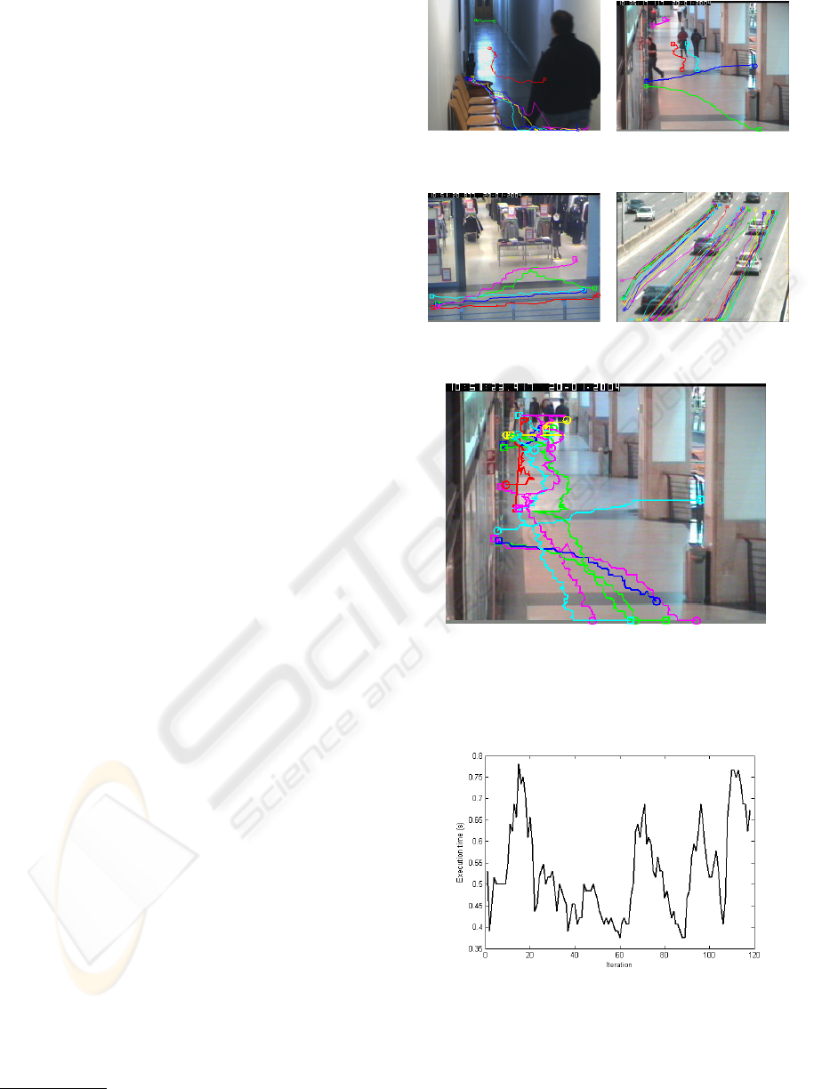
Figure 1 shows the obtained paths. We tested se-
quences from the CAVIAR dataset
5
, and used the sup-
plied labelings as detections. The sequence Corri-
dor was captured independently for our purpose, and
detections for the Highway sequence were obtained
with an object segmentation system under develop-
ment at our laboratory. Note that the sequence Walk-
ByShop1cor (CAVIAR) is very challenging: there are
11318 detections over 2360 frames of video. Such
a long video would require significant computational
resources if analized directly with a global method; so
it is the perfect test subject for our continuous tracking
scheme. With a window size of 60 frames and updat-
ing the window every 20 frames ( f = 20), we’re able
to track objects even in the presence of long occlu-
sions (see the cyan track that passes behind the pillar
in Figure 1e). The missed tracks are accounted for by
the pack of barely visible people far away from the
camera.
Note that there was no parameter tuning for each
different sequence. The tracker is robust against its
own parameters. For each scene we had to supply a
map of the entry/exit locations and scene occlusions,
which was done by hand but could be learned over
time as in (Huang et al., 2008). We also had to find
the covariance matrices for all the Gaussian models
using training data, but they have similar values for
all scenes; the exception is the Highway scene, where
tracked cars have obviously different characteristics
from people tracked in other videos (namely the ap-
pearance variance, which is lower).
Figure 2 presents a plot of the running time per
iteration for the WalkByShop1cor sequence. The sys-
tem is able to run in real-time, since calculations for
a batch of detections are done well before the next
batch arrives.
6 CONCLUSIONS
Despite the superior performance of trackers based
on global optimization methods, to this day they
have been restricted to lab use due to their inherent
need for complete knowledge of the scene, which is
not feasible for 24 hours-a-day operation. The pro-
5
http://homepages.inf.ed.ac.uk/rbf/CAVIARDATA1/
(a) Corridor sequence. (b) EnterExitCrossing-
Paths1cor sequence.
(c) WalkByShop1front
sequence.
(d) Highway sequence.
(e) WalkByShop1cor sequence.
Figure 1: Resulting paths of each scene, superimposed on
an example frame. The positions shown are always at the
bottom-center of each detection’s bounding box (i.e., an es-
timate of its position on the ground).
Figure 2: Execution time per iteration in the Walk-
ByShop1cor sequence. Note that each iteration goes
through 2 seconds of video (20 frames), but each one is pro-
cessed in under 1 second in this complicated sequence.
posed method allows them to operate continuously.
We show encouraging results from different datasets,
VISAPP 2010 - International Conference on Computer Vision Theory and Applications
214

tracking both cars and pedestrians, without tuning the
tracker’s parameters for each set. The system is able
to run in real-time, showing the flexibility of the ap-
proach and the discriminative power of Region Co-
variance Matrices. Hopefully we’ve been able to fit
the missing link that will enable the adoption of global
optimization methods in real-world tracking applica-
tions.
REFERENCES
Ahuja, R. K. (2008). Network flows. PhD thesis, Mas-
sachusetts Institute of Technology, Cambridge.
Betke, M., Hirsh, D. E., Bagchi, A., Hristov, N. I., Makris,
N. C., and Kunz, T. H. (2007). Tracking large variable
numbers of objects in clutter. Proceedings of the IEEE
Computer Society June.
Huang, C., Wu, B., and Nevatia, R. (2008). Robust ob-
ject tracking by hierarchical association of detection
responses. In Proceedings of the 10th European Con-
ference on Computer Vision: Part II, page 801.
Huang, T. and Russell, S. (1997). Object identification
in a bayesian context. In International Joint Con-
ference on Artificial Intelligence, volume 15, pages
1276–1283.
Javed, O., Rasheed, Z., Shafique, K., and Shah, M. (2003).
Tracking across multiple cameras with disjoint views.
In Ninth IEEE International Conference on Computer
Vision, 2003. Proceedings, pages 952–957.
Kuhn, H. W. (1955). The hungarian method for the assign-
ment problem. Naval Research Logistics Quarterly,
2:83–97.
Li, K., Miller, E. D., Chen, M., Kanade, T., Weiss, L. E.,
and Campbell, P. G. (2008). Cell population tracking
and lineage construction with spatiotemporal context.
Medical Image Analysis, 12(5):546–566.
Mills-Tettey, G. A., Stentz, A., and Dias, M. B. (2007).
The Dynamic Hungarian Algorithm for the Assign-
ment Problem with Changing Costs. Citeseer.
Okuma, K., Taleghani, A., Freitas, N. D., Little, J. J., and
Lowe, D. G. (2004). A boosted particle filter: Multi-
target detection and tracking. Lecture Notes in Com-
puter Science, pages 28–39.
Palaio, H. and Batista, J. (2008). A region covariance em-
bedded in a particle filter for multi-objects tracking.
Porikli, F., Tuzel, O., and Meer, P. (2006). Covariance track-
ing using model update based on means on riemannian
manifolds. Proc. IEEE Conf. on Computer Vision and
Pattern Recognition.
Reid, D. B. (1979). An algorithm for tracking multiple
targets. IEEE Transactions on Automatic Control,
24(6):843–854.
Shafique, K. and Shah, M. (2005). A noniterative greedy
algorithm for multiframe point correspondence. IEEE
transactions on pattern analysis and machine intelli-
gence, 27(1):51–65.
Stauffer, C. (2003). Estimating tracking sources and sinks.
In Computer Vision and Pattern Recognition Work-
shop, 2003. CVPRW’03. Conference on, volume 4.
Taj, M., Maggio, E., and Cavallaro, A. (2007). Multi-
feature graph-based object tracking. Lecture Notes in
Computer Science, 4122:190.
Tuzel, O., Porikli, F., and Meer, P. (2008). Pedestrian detec-
tion via classification on riemannian manifolds. IEEE
Transactions on Pattern Analysis and Machine Intel-
ligence, pages 1713–1727.
DYNAMIC GLOBAL OPTIMIZATION FRAMEWORK FOR REAL-TIME TRACKING
215
