
TOWARDS GENERIC FITTING USING DISCRIMINATIVE ACTIVE
APPEARANCE MODELS EMBEDDED ON A RIEMANNIAN
MANIFOLD
Pedro Martins and Jorge Batista
∗
ISR-Institute of Systems and Robotics, Dep. of Electrical Engineering and Computers
FCTUC-University of Coimbra, Coimbra, Portugal
Keywords:
Active appearance models, Discriminative fitting, Riemannian manifolds.
Abstract:
A solution for Discriminative Active Appearance Models is proposed. The model consists in a set of de-
scriptors which are covariances of multiple features evaluated over the neighborhood of the landmarks whose
locations are governed by a Point Distribution Model (PDM). The covariance matrices are a special set of
tensors that lie on a Riemannian manifold, which make it possible to measure the dissimilarity and to update
them, imposing the temporal appearance consistency. The discriminative fitting method produce patch re-
sponse maps found by convolution around the current landmark position. Since the minimum of the responce
map isn’t always the correct solution due to detection ambiguities, our method finds candidates to solutions
based on a mean-shift algorithm, followed by an unsupervised clustering technique used to locate and group
the candidates. A mahalanobis based metric is used to select the best solution that is consistent with the PDM.
Finally the global PDM optimization step is performed using a weighted least-squares warp update, based on
the Lucas and Kanade framework. The weights were extracted from a landmark matching score statistics. The
effectiveness of the proposed approach was evaluated on unseen data on the challenging Talking Face video
sequence, demonstrating the improvement in performance.
1 INTRODUCTION
Facial image alignment is the key aspect in many
computer vision applications, such as tracking and
recognition. In the past years, most existing meth-
ods have used generative based methods, where
the shape and texture variation were learned from
training images. The Active Appearance Models
(AAM)(T.F.Cootes et al., 2001)(Matthews and Baker,
2004) is one of the most effective techniques with
respect to fitting accuracy and efficiency. Although,
it consists on generative holistic representations (in
sense that all pixels belonging to the object are used).
Due to the generative nature, AAM is able to synthe-
size a high quality model where the data is used si-
multaneously during the fitting, producing a high ac-
curacy fitting. This representation generalization per-
forms poorly when the target exhibits large amounts
of variability, such as the case of the human face un-
der variations of identity, expression, pose, lighting or
non-rigid motion due to the huge dimensional repre-
∗
Work funded by FCT grant SFRH/BD/45178/2008.
sentation of the appearance (learnt from limited data).
The main drawback with the generative approaches
is that typically they only work well for the individ-
uals held in the training dataset(Gross et al., 2005)
due to the fact that the appearance is eigen based
and captured by a linear Principal Components Anal-
ysis (PCA). Various solutions were proposed to deal
with this limitation: Adaptive AAM(Batur and Hayes,
2005), Constrained AAM, that are mainly based on
online updating the Jacobian matrix. Other Adap-
tive AAM solutions (Sung and Kim, 2009) (Matthews
et al., 2004) consist on online incremental PCA.
Recently, discriminative based methods such as the
Constrained Local Model (CLM)(D.Cristinacce and
T.F.Cootes, 2008) or (Wang et al., 2008a) (Wang
et al., 2008b) have been proposed. These methods
use a set of discriminative template regions surround-
ing individual landmarks whose locations are gov-
erned by a Point Distribution Model (PDM). The fit-
ting is based on an exhaustive local search around the
current landmark location, producing response maps
(for each landmark) and driving the parameters of the
PDM in order to maximize the sum of responses for
363
Martins P. and Batista J. (2010).
TOWARDS GENERIC FITTING USING DISCRIMINATIVE ACTIVE APPEARANCE MODELS EMBEDDED ON A RIEMANNIAN MANIFOLD.
In Proceedings of the International Conference on Computer Vision Theory and Applications, pages 363-369
DOI: 10.5220/0002823603630369
Copyright
c
SciTePress
each point. Compared with the holistic representa-
tions, such as AAM, working at patch level offers ex-
tra flexibilities. The parts-based representation im-
prove the model’s representation capacity, as it ac-
counts only for local correlations between pixel val-
ues and naturally is presents good performance in fit-
ting unseen appearances in comparison with the lead-
ing holistic approaches. The CLM uses as patch de-
scriptors, normalized correlation response surfaces.
In (Wang et al., 2008a) (Wang et al., 2008b) the dis-
criminant descriptor is obtained using machine learn-
ing methods, i.e. a linear Support Vector Machines
(SVM), which require a extensive training, labeling
lots of positive and negative samples. Our approach
fits on the discriminative class of methods where, like
the standard AAM, consists in two separated mod-
els: the shape and the appearance models. The shape
model is an ordinary PDM that deals with the posi-
tion of the landmarks. The appearance is composed
by a set of descriptors for each of the landmarks in
the PDM. The descriptors are covariance matrices of
multiple features evaluated on the surrounding loca-
tion of the landmarks. Since the covariance matrices
are a special set of tensors that lie on a Riemannian
manifold, it is possible to measure the dissimilarity
between two covariances, and also to update them,
imposing the temporal appearance consistency. The
method starts using a generic covariance (the aver-
age covariance observed in the training set) which is
then continuously updated. Although, like the pre-
vious methods (D.Cristinacce and T.F.Cootes, 2008)
(Wang et al., 2008a) (Wang et al., 2008b), the patch
response maps found by convolution around the cur-
rent landmark position suffers from detection ambi-
guities. It will be shown that the minimum (in covari-
ance dissimilarity) of the responce map isn’t always
the desired solution. A solution based on a mean-
shift algorithm is proposed, finding candidates to so-
lutions, followed by an unsupervised clustering tech-
nique(Figueiredo and Jain, 2002) locating and group-
ing the candidates. A mahalanobis based metric is
used to select the best solution consistent with the
PDM. Finally the global optimization step, solving
the PDM is performed using a weighted least-squares
warp update based on the Lucas and Kanade frame-
work(Baker and Matthews, 2004). The weights were
extracted from landmark matching score statistics.
This paper is organizedas follows: section 2 describes
background subjects required, namely the basics on
Riemann Manifolds and PDM building. In section 3
our approach is detailed presented, section 4 presents
experimental results and in section 5 conclusions are
presented.
2 BACKGROUND
2.1 Shape Model
The shape of a (2D) Point Distribution Model (PDM)
is defined by the vertex locations of a mesh. The rep-
resentation used for a single v-point shape is a 2v vec-
tor given by s = (x
1
, . . . , x
v
, y
1
, . . . , y
v
)
T
. The PDM
training data consists of a set of annotated images
with the shape mesh marked (usually by hand). All
the shapes are then aligned to a common mean shape
using a Generalised Procrustes Analysis (GPA), re-
moving location, scale and rotation effects. Princi-
pal Components Analysis (PCA) are then applied to
the aligned shapes, resulting on the linear parametric
model s = s
0
+ Φp, where new shapes, s, are syn-
thesized by deforming the mean shape, s
0
, using a
weighted linear combination of eigenvectors, φ
i
, i =
1, . . . , n. n is the number of eigenvectors that holds
a user defined variance, typically 95%. p is a vec-
tor of shape parameters which represents the weights.
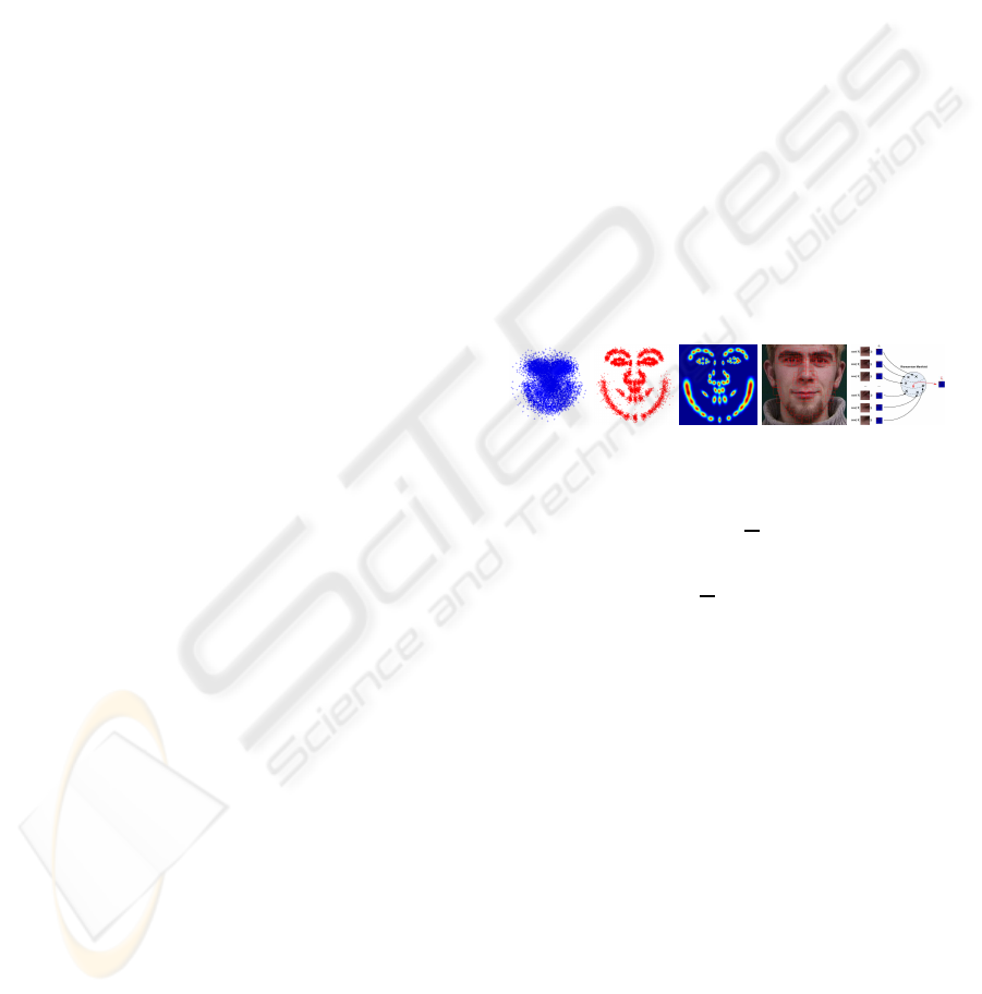
See Figure 1-a)b)c). Notice that the GPA makes that
(a) (b) (c) (d) (e)
Figure 1: a) Shape raw data. b) Aligned landMarks after
GPA. c) Shape covariance Σ
k
around each landmark. d)
Patches P
k
, l × l around each landmark. e) Illustration of
finding the average covariance C
k
for a specific patch (left
side of left eye corner). Each training image provide a nor-
malized patch. The covariances for the feature vector f are
evaluated and using eq.2, C
k
is found.
the PDM do not model the similarity transformation
which is required onto the target image. To overcome
this we use the approach proposed by (Matthews and
Baker, 2004), i.e., we include a special set of 4 eigen-
vectors ψ
1
, . . . , φ
4
. A full shape is then described
by a linear system s = s
0
+
∑
n
i=1
p
i
φ
i
+
∑
4
j=1
q
j
ψ
j
where q represents the 2D pose parameters with q
1
=
scos(θ) − 1, q
2
= ssin(θ), q
3
= t
x
, q
4
= t
y
where s,
θ, (t
x
, t
y
) represents the scale, rotation and translation
w.r.t. the base mesh s
0
.
2.2 Texture Model - Covariance of
Features
The discriminative appearance model used is based
on a descriptor of the texture around each one of the
v landmarks. Inspired on the work of (Porikli et al.,
2006), a quadrangular region P (patch) with size l is
VISAPP 2010 - International Conference on Computer Vision Theory and Applications
364

sampled around each landmark. See Figure 1-d. On
each of the regions, P
k
, k = 1, . . . , v, several features
f are extracted for each pixel x = (x, y)
T
, ∈ P
k
where
f = [x y I
x
I
y
q
I
2
x
+ I
2
y
arctan
I
y
I
x
I
xx
+ I
yy
].
The features used are the pixel position (x, y), hori-
zontal and vertical gradients (I
x
, I
y
), gradient magni-
tude, gradient phase, and the Laplacian. The main
advantages of our formulation is that it can always
allow more features in order to find a better descrip-
tor for P
k
without changing the remaining formula-
tion. Stacking all measures of f, i.e. F
k
= f ∈ P
k
, the
d × d covariance matrix for the features is given by
C
k
=
1
l
2
−1
∑
l
2
i=1
(F
k
i
− µ
P
k
)(F
k
i
− µ
P
k
)
T
where µ
P
k
is
the vector of feature means within the region P
k
. The
covariance C
k
is used as region descriptor (which rep-
resents the correlations between the features f for the
entire region P
k
). The main advantage of using co-
variances of features is that, if they are positive defi-
nite matrices, C
k
lie in a Riemannian Manifold and is
possible to measure dissimilarities and make updates.
2.2.1 Dissimilarity between Covariances
The covariance matrices do not lie on Euclidean
space. Based on the Riemannian invariants, a distance
metric(Pennec et al., 2006) is used. The dissimilarity
between two covariances matrices C
1
and C
2
is given
by
ρ(C
1
, C
2
) =
s
m
∑
i=1
λ
i
(C
1
, C
2
) (1)
where λ
i
(C
1
, C
2
)
i=1,...,m
are the generalized eigenval-
ues of C
1
and C
2
, computed from λ
i
C
1
x
i
− C
2
x
i
=
0, i = 1, ..., d and x
i
6= 0 are the generalized eigenvec-
tors. Note that ρ(C
1
, C
2
) ≥ 0.
2.2.2 Updating Covariances - Finding C
k
The mean of the points on the manifold minimizes
the L
2
norm of C = argmin
∑
T
t=1
ρ
2
(C, C
t
). (Pennec
et al., 2006) proposed a gradient descent approach to
compute the C by C
i+1
= exp
C
i
1
T
∑
T
t=1
log
C
i
(C
t
)
.
To prevent the model from contamination, it is possi-
ble to weight the data points by a factor proportional
to its similarity to the current model, resulting
C
i+1
= exp
C
i
1
ρ
∗
T
∑
t=1
ρ
−1
(C
t
, C
∗
)log
C
i
(C
t
)
!
(2)
where ρ is defined in eq.1, ρ
∗
=
∑
T
t=1
ρ
−1
(C
t
, C
∗
) and
C
∗
is the model computed at the T previous frames.
Each training image provide a set of v covariances
matrices, C
k
(for each landmark k). For N images
in the set, the average covariance matrix, C
k
, is com-
puted over the Riemannian Manifold using eq.2. See
Figure 1-e for a graphical interpretation of this pro-
cess. The mean covariance, C
k
, is used as the initial
descriptor for that specific landmark k.
2.3 Image Normalization - Affine Warp
Since the covariance isn’t invariant to scale and ro-
tation effects, a normalization at image level is re-
quired. The normalization is based on an affine warp
of the entire image in a way that the current mesh s is
mapped into the reference base mesh s
0
. At a glance,
it seems that a similarity warp will be sufficient due to
the nature of this problem, but experimentally it was
concluded that the two extra degrees of freedom of
the affine model provide a better quality in covariance
matching.
3 OUR APPROACH - DAAM-R
After building the PDM and evaluating the average
covariance C
k
for each landmark k (in a training
stage), fitting the Discriminative AAM embedded on
a Riemannian Manifold (DAAM-R) consists on find-
ing k local optimal displacements, ∆x
†
, from the PDM
current mesh position s. The local updates, expressed
in the base mesh, will be constrained to lie in the
subspace spanned by Φ by an nonlinear optimization
based on the Lucas Kanade framework(Baker et al.,
2003). (See section 3.1). The goal is to find the devi-
ation from the PDM, ∆x, for each landmark. The se-
quential steps of proposed approach are enumerated
and Figure 2 shows the overall view for the fitting
methodology. (1) Scanning by convolution around
a local region finding a response map of covariances
dissimilarities (Figure 2-a). (2) The minimum of the
responce map, i.e. the lower dissimilarity, doesn’t
always correspond to the correct landmark location.
Actually, in some cases it can be a poor estimate,
since the features consists of small image patches that
often contain limited structure, leading to detection
ambiguities. It is however assumed that the correct
solution is a local minima. A modified version of a
mean-shift algorithm (section 3.2) is used to detect all
the local minima (see Figure 2-b) providing a set of
candidates to the landmark solution. (3) The mean-
shift will produce clusters with the candidates to so-
lutions, ∆x
∗
k
. At this stage is important to define the
number and location of these clusters. For this pro-
pose an unsupervised clustering method proposed by
TOWARDS GENERIC FITTING USING DISCRIMINATIVE ACTIVE APPEARANCE MODELS EMBEDDED ON A
RIEMANNIAN MANIFOLD
365
(Figueiredo and Jain, 2002) it is used. See Figure 2-c
and section 3.3. (4) Knowing the clusters and their
locations, it is required to select the best cluster, ∆x
†
k
,
section 3.4. The selection is based on the cluster that
will be more consistent with the PDM (Figure 2-d).
(5) Finally, establish the landmark matching score as-
signing weights to the foundsolution (section 3.5) and
performing global PDM optimization (section 3.1).
2 4 6 8 10 12 14 16 18 20
2
4
6
8
10
12
14
16
18
20
370
375
380
385
390
190
195
200
205
210
215
0
0.5
1
1.5
2
2.5
2 4 6 8 10 12 14 16 18 20
2
4
6
8
10
12
14
16
18
20
250
255
260
265
270
275
225
230
235
240
245
0
0.5
1
1.5
2
2.5
3
2 4 6 8 10 12 14 16 18 20
2
4
6
8
10
12
14
16
18
20
220
225
230
235
240
245
290
295
300
305
310
315
0
0.5
1
1.5
2
2.5
3
2 4 6 8 10 12 14 16 18 20
2
4
6
8
10
12
14
16
18
20
(a)
315
320
325
330
335
340
390
395
400
405
410
0
1
2
3
4
5
6
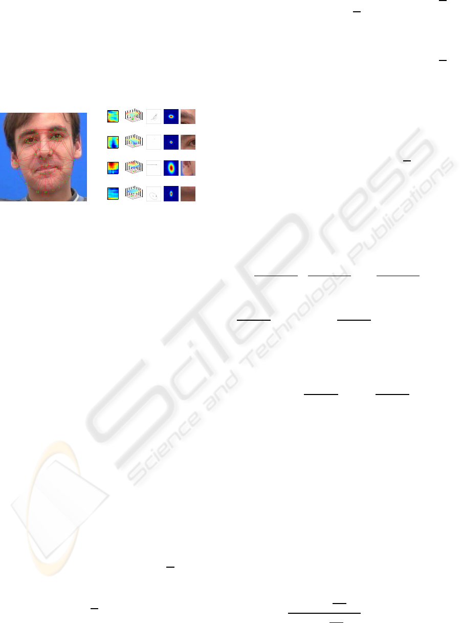
(b) (c) (d) (e)
Figure 2: Overview of the DAAM-R. The left main figure
represents the first iteration of the method. Starting with an
initial estimate of the position of the face (by AdaBoost).
a) Response maps of covariance of features dissimilarity
around each x
k
(blue small dissimilarity). b) 3D mesh for
the response maps. At the ground level with red color is
represented the mean-shift seeds starting grid. The green
circles are the seeds final position (local minima). c) Unsu-
pervised clustering to find the clusters and their locations.
The red cross at the center represents the current landmark
position x
k
. The small green circles are the mean-shift seeds
at a near local minima location and the ellipses are the clus-
ters found. d) Representation for Σ
k
. e) Detailed matching
solutions. The green dots are the centroid locations, x
∗
k
i
,
and the selected solution x
†
k
is the one pointed by the green
arrow.
3.1 Global Optimization - Fitting the
PDM
The PDM fitting is accomplish using the Lucas and
Kanade framework(Baker and Matthews, 2004). The
warp function is given by
W(x, p, q) = s
0
+ Φp+ Ψq (3)
where p is the shape parameters and q the similarity
parameters. The non-rigid alignment can be posed
into the following optimization problem
argmin
p,q
v
∑
k=1
ρ(C
k
{s
0
+ Φp+ Ψq}), C
∗
k
) (4)
minimizing the covariance dissimilarity ρ(.) between
the model covariance, C
∗
k
, and the covariance com-
puted on a shifted location, but constrained to be con-
sisted with the PDM, C
k
{s
0
+ Φp+ Ψq}), for all the
v patches in the model. The model covariance, C
∗
k
,
starts by being the average C
k
on the Manifold. Is
computed from the training images and is weighted
updated every frame enforcing the temporal appear-
ance consistency using the approach described in sec-
tion 2.2.2. A T sized buffer is used to evaluate C
∗
k
.
This update process is only done after the PDM fitting
of the target frame. For solving the cost function eq.
4, a weighted least-squares optimization, proposed by
(Wang et al., 2008a), is used. It requires finding v
local translations by exhaustively search the region
around each patch such that
∆x
†
k
= argmin
∆x
k
ρ(C
k
{x
k
+ ∆x
k
}), C
∗
k
) (5)
where ∆x
†
k
is the optimal, in some sense, local dis-
placement for the patch k. The evaluation of ∆x
†
k
is
described on the following subsections. The weighted
least-squares warp update is given by
∆p =
∂W(x, p, q)
∂p
W
∂W(x, p, q)
∂p
T
!
−1
∂W(x, p, q)
∂p
W∆x
†
(6)
where the Jacobian of the warp is given by
∂W(x,p,q)
∂p
= Φ
T
and
∂W(x,p,q)
∂q
= Ψ
T
. W is
a 2v × 2v diagonal matrix of weights, W =
diag(w
1
, ..., w
v
, w
1
, ..., w
v
). Each w
k
weight, measures
the fitting importance for landmark k. See section 3.5
for details in how to estimate the weights. The pa-
rameters update equation for ∆q is similar to eq.6 but
insted of using
∂W(x,p,q)
∂p
it uses
∂W(x,p,q)
∂q
. For this
particular case the Jacobian of the warp is constant,
and the forward additive update method(Baker and
Matthews, 2004) can be used. Solving the PDM con-
sists in iteratively use eq.6 and update the parameters
by p ← p+ ∆p and q ← q + ∆q until k∆pk ≤ ε, or a
maximum number of iterations is reached. Note that
the image normalization process, described earlyer in
section 2.3, is performed at each iteration.
3.2 Weighted Mean-Shift - Find
Candidates
Mean-shift algorithm is a robust clustering technique
which does not require prior knowledge on the num-
ber of clusters(Comaniciu and Meer, 2002). The
weighted mean shift vector at point x is defined
as m
h
(x) =
∑
m
i=1
w
i
x
i
g
x−x
i
h
2
∑
m
i=1
w
i
g
x−x
i
h
2
where g(s) = −k
′
(s),
with k(s) being the kernel profile (it is used k(s) =
VISAPP 2010 - International Conference on Computer Vision Theory and Applications
366

e
−
s
2
) and the h bandwidth. w
i
is the normalized
weight assigned to each data point x
i
. The algo-
rithm starts at the data points and at each iteration
t moves in the direction of the mean shift vector
x
t+1
= x
t
+ m
h
(x
t
). The mean-shift vector always
points toward the direction of the maximum increase
in the density. If weights are assigned as w
i,i=1,...,m
=
ρ
−1
(C
k
{x
k
+ ∆x
k
}, C
∗
k
), where m is the number of
seeds (i.e. equal to the inverse of the dissimilarity
of the response maps), the seeds will move into the
local minima. Note that the weights, w
i
, should be
normalized such that
∑
m
i=1
w
i
= 1. The selection of
the number and the starting position of the seeds is
very important. A sparse grid of 3× 3 blocks is used,
where a single seed is assigned to the position inside
the block that has the higher weight. The number of
seeds used, m, will be the number of 3× 3 blocks in-
side the grid of the scanned areas.
3.3 Finding Clusters
The mean-shift will provide candidates to solutions.
Searching for those candidates is a clustering prob-
lem. For this propose the unsupervised clustering
method proposed by (Figueiredo and Jain, 2002) was
used. Usually the mean-shift seeds converge around
a few locations, forming clusters where the seeds are
not positioned at the exact same place. The clustering
also filters this effect by taking the centroid position
as the candidate solution.
3.4 Selecting the Best Cluster
Knowing the clusters and their centroid locations it
is required to select the best cluster. The selection
is based on the cluster that is more consistent with
the PDM. Recalling Figure 1-c, the individual shape
localization covariance, Σ
k
, was estimated. The se-
lected cluster is the one that has the lower maha-
lanobis distance w.r.t. the correspondent PDM land-
mark. Formally, the centroid locations x
∗
k
i
are given
by x
∗
k
i
= x
k
+ ∆x
∗
k
i
with i = 1, . . . , c, and c the num-
ber of centroids found. The deviation update found
for each cluster is ∆x
∗
k
i
. The selected candidate for
the solution, x
†
k
, is the one that has the lower maha-
lanobis distance, i.e. is more close to the PDM dis-
tribution x
†
k
= argmind
m
(x
∗
k
i
, Σ
k
), where d
m
(.) is the
mahalanobis distance that is evaluated for all x
∗
k
i
, and
Σ
k
is the shape position covariance of the landmark k.
3.5 Landmark Matching Score
The PDM optimization is based on a weighted least-
square warp update, dealing with some possible land-
marks mismatches. From eq.6 this information is
included as a diagonal matrix of weights and those
weights are based on landmark confidences. The
statistics for the landmarks covariance of features
matching score can be learnt previously from the
training images. The residual error on matching, C
k
,
follows a half normal which is approximated by a
normal distribution with zero mean and a given stan-
dard deviation ∼ N (0, σ
C
k
). The error standard de-
viation σ
C
k
can be estimated from the training set
as σ
C
k
=
q
∑
N
i=1
ρ(C
i
,C
k
)
2
N−1
, where N is the total num-
ber of images. Knowing σ
C
k
and defining C
†
k
to be
the covariance of features evaluated at the solution
x
†
k
, the weights for the matrix W can be assigned as
w
k
= exp
−
ρ(C
†
k
,C
∗
k
)
2
2σ
C
k
.
4 EXPERIMENTAL RESULTS
The experimental results were conducted using two
free available independent datasets. The IMM
dataset
2
annotated with v = 58 landmarks, see Fig-
ure 1-a and the FGNet Talking Face sequence (TF).
The main experience consists on training the DAAM-
R with about 160 near frontal images from the IMM
set and test the ability of fitting in unseen images,
comparing it with other fitting algorithms trained with
the same input data. The DAAM-R training consists
in building the PDM, compute the average covariance
of features for each landmark, C
k
, and find the match-
ing statistics σ
C
k
using only the images from the IMM
set. The fitting accuracy is evaluated using the ini-
tial 1000 frames of the TF sequence. Our method
(DAAM-R) is compared with the standard AAM al-
gorithms: the Project Out (PO)(Matthews and Baker,
2004), the Simultaneous Inverse Compositional (SIC)
and the SIC Efficient Approximation (SIC-EA)(Baker
et al., 2003). The method is also tested against the
robust extensions: Roboust Normalization Inverse
Compositional (RNIC)(Baker et al., 2003) and the
Roboust SIC (RSIC)(Baker et al., 2003). Regarding
the remaining details about the DAAM-R, the sam-
pled patches P
k
have the size of 11 × 11, (l = 11),
(intraocular distance of about 80 pixels). Durring the
fitting process the search area is a window of 21× 21
pixels around each landmark. For the mean-shift,
2
www2.imm.dtu.dk/ aam
TOWARDS GENERIC FITTING USING DISCRIMINATIVE ACTIVE APPEARANCE MODELS EMBEDDED ON A
RIEMANNIAN MANIFOLD
367
the system works well with a bandwidth of h = 8,
ε = 0.01, and maximum number of iterations 50. The
number of seeds used were m = 49. The unsupervised
clustering requires the minimal and maximal number
of clusters to find, 1 and 5 respectively. The model
covariance buffer is T = 30, which means that that
for every landmark the C
∗
k
is computed from 30 pre-
vious weighted samples. The termination criteria in
DAAM-R was set to ε = 0.75 and the maximum iter-
ations was set to 10. For the other algorithms ε = 0.75
and maximum iterations of 20. The robust algorithms
also require the choose of a error norm, the Talwar
function is used (gives a weight of 1 to inliers and 0 to
outliers), where the scale parameter is estimated from
the error image assuming that there exists 15% of out-
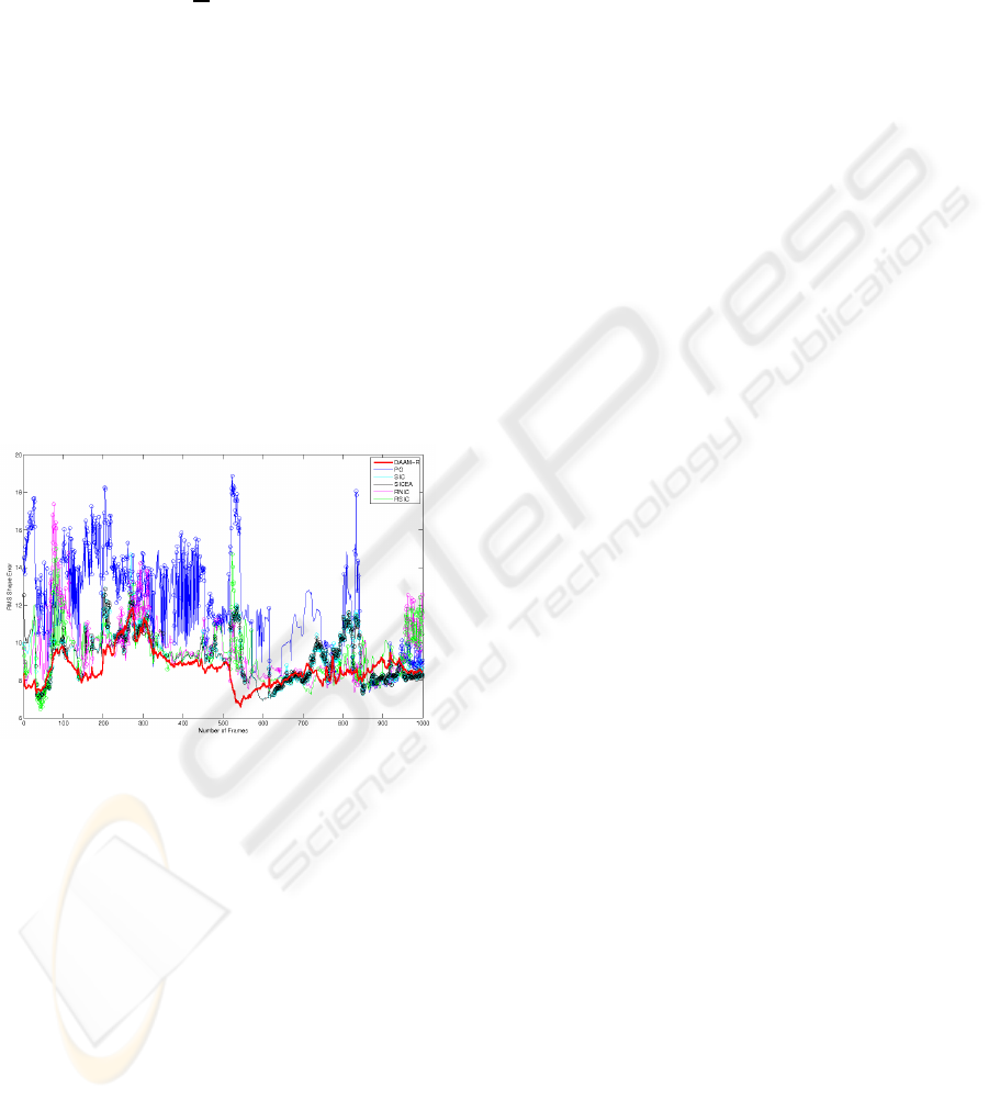
liers. The Figure 3 shows the RMS fitting error in the
TF sequence for all the evaluated methods. Since the
IMM uses a 58 landmark scheme and the TF uses 68,
the error was only measured over the correspondent
landmarks. The colored circles over the graphic rep-
resent reinitializations of the models. Note that our
approach, DAAM-R, never make a restart. The re-
sults show that the method is generally very accurate.
Figure 3: Top figures are the fitted frames 1 and 500 of the
Talking Face sequence for every algorithms. At bottom the
RMS error in fitting the first 1000 frames of the Talking
Face video sequence (unseen data). Best viewed in color.
5 CONCLUSIONS
The DAAM-R uses independent shape and texture
models. The texture is composed by a set descriptors
for the landmarks. These descriptors are covariances
of multiple features evaluated around the landmark
locations which is governed by a PDM. The covari-
ance matrices lie on a Riemannian manifold, which
make possible to measure the dissimilarity and to up-
date them, imposing the temporal appearance consis-
tency. Using a discriminative fashion fitting approach,
response maps are found. Since the minimum of the
responce map isn’t always the correct solution a strat-
egy based on mean-shift is used to find candidates to
solutions (local minima). An unsupervised cluster-
ing technique is used to locate and group the candi-
dates and a mahalanobis based metric is used to se-
lect the best solution consistent with the PDM. The
global optimization for the PDM is performed using
a weighted least-squares warp update, where weights
were extracted from the landmark matching confi-
dences statistics. The DAAM-R trained with mostly
frontal images taken from the IMM dataset is evalu-
ated by fitting to unseen data on the challenging Talk-
ing Face video sequence (1000 frames). The model
performs well without lose track during all the se-
quence. As future work we propose to used the mean-
shift using an adaptive bandwith, improving the so-
lution section and a evaluation for the quality of the
selected vector of features. As a final note, the en-
tire process can be speeded up using the integral im-
age covariance computation and is suitable for paral-
lel computing since the response patches for the land-
marks are independent.
REFERENCES
Baker, S. and Matthews, I. (2004). Lucas-kanade 20 years
on: A unifying framework. International Journal of
Computer Vision, 56(1):221 – 255.
Baker, S., R.Gross, and I.Matthews (2003). Lucas kanade
20 years on: A unifying framework: Part 3. Technical
report, CMU Robotics Institute.
Batur, A. and Hayes, M. (2005). Adaptive active appearance
models. IEEE Transactions on Image Processing.
Comaniciu, D. and Meer, P. (2002). Mean shift: A robust
approach toward feature space analysis. IEEE PAMI.
D.Cristinacce and T.F.Cootes (2008). Automatic feature
localisation with constrained local models. Pattern
Recognition.
Figueiredo, M. A. and Jain, A. K. (2002). Unsupervised
learning of finite mixture models. IEEE PAMI.
Gross, R., Matthews, I., and Baker, S. (2005). Generic vs.
person specific active appearance models. Image and
Vision Computing, 23(1):1080–1093.
Matthews, I. and Baker, S. (2004). Active appearance mod-
els revisited. IJCV.
Matthews, I., Ishikawa, T., and Baker, S. (2004). The tem-
plate update problem. IEEE Transactions on Pattern
Analysis and Machine Intelligence, 26(1):810 – 815.
Pennec, X., Fillard, P., and Ayache, N. (2006). A rieman-
nian framework for tensor computing. IJCV.
Porikli, F., Tuzel, O., and Meer, P. (2006). Covariance track-
ing using model update based on lie algebra. In IEEE
CVPR.
Sung, J. and Kim, D. (2009). Adaptive active appearance
model with incremental learning. Pattern Recognition
Letters.
VISAPP 2010 - International Conference on Computer Vision Theory and Applications
368

T.F.Cootes, Edwards, G., and C.J.Taylor (2001). Active ap-
pearance models. IEEE PAMI.
Wang, Y., Lucey, S., and Cohn, J. (2008a). Enforcing con-
vexity for improved alignment with constrained local
models. In IEEE CVPR.
Wang, Y., Lucey, S., Cohn, J., and Saragih, J. M. (2008b).
Non-rigid face tracking with local appearance consis-
tency constraint. In IEEE Automatic Face and Gesture
Recognition.
TOWARDS GENERIC FITTING USING DISCRIMINATIVE ACTIVE APPEARANCE MODELS EMBEDDED ON A
RIEMANNIAN MANIFOLD
369
