
A GEOMETRIC APPROACH TO CURVATURE ESTIMATION ON
TRIANGULATED 3D SHAPES
Mohammed Mostefa Mesmoudi, Leila De Floriani and Paola Magillo
Department of Computer Science and Information Science (DISI), University of Genova
Via Dodecaneso 35, 16146 Genova, Italy
Keywords:
Gaussian and mean curvatures, Surface meshes.
Abstract:
We present a geometric approach to define discrete normal, principal, Gaussian and mean curvatures, that
we call Ccurvature. Our approach is based on the notion of concentrated curvature of a polygonal line and
a simulation of rotation of the normal plane of the surface at a point. The advantages of our approach is its
simplicity and its natural meaning. A comparison with widely-used discrete methods is presented.
1 INTRODUCTION
Curvature is one of the main important notions used
to study the geometry and the topology of a surface.
In combinatorial geometry, many attempts to define a
discrete equivalent of Gaussian and mean curvatures
have been developed for polyhedral surfaces (Gatzke
and Grimm, 2006; Surazhsky et al., 2003). Dis-
crete approaches include smooth approximations of
the surface using interpolation techniques (Hahmann
et al., 2007), and approaches that deal directly with
the mesh (Meyer et al., 2003; Taubin, 1995; Watanabe
and Belyaev, 2001). All the methods are not satisfac-
tory in what concerns approximation errors, control,
and convergence when refining a mesh (Borrelli et al.,
2003; Surazhsky et al., 2003; Xu, 2006).
In the fifties, Aleksandrov introduced concen-
trated curvature as an intrinsic curvature measure for
polygonal surfaces (Aleksandrov, 1957). This tech-
nique has been used in the geometric modeling com-
munity under the name of angle defect method (Al-
boul et al., 2005; Akleman and Chen, 2006). Con-
centrated curvature does not suffer from the problems
linked to errors and and their control, and satisfies a
discrete analogous version of the well known Gauss-
Bonnet theorem. However, Concentrated curvature
depends weakly on the local geometric shape of the
surface.
Here, we use Aleksandrov’s idea to define con-
centrated curvature for polygonal lines. We prove in
such a case that concentrated curvature is an intrin-
sic measure that is expressed using only the fracture
angle of the polygonal line at its vertices. We then
define a discrete normal curvature of a polygonal sur-
face at a vertex. We simulate the rotation of normal
planes to define principal curvatures and, thus, obtain
new discrete estimators for Gaussian and mean curva-
tures. We call all such curvatures Ccurvatures, since
they are obtained as generalization to surfaces of the
concept of concentrated curvature for polygonal lines
just introduced. The major advantage of this method
is the use of intrinsic properties of a discrete mesh to
define geometric features that have the same proper-
ties as the analytic methods. In this work, we also
compare Gaussian and mean Ccurvatures with widely
used discrete curvature estimators for analytic Gaus-
sian and mean curvatures and with concentrated cur-
vature (according to Aleksandrov’s definition).
2 BACKGROUND NOTIONS
In this Section, we briefly review some fundamental
notions on curvature in the analytic case and on con-
centrated curvature.
Let C be a smooth curve having parametric repre-
sentation (c(t))
t∈R
. The curvature k(p) of C at a point
p = c(t
0
) is given by
k(p) =
1
ρ
=
|c
0
(t) ∧ c”(t)|
|c
0
(t)|
3
,
where ρ is called the curvature radius. Number ρ cor-
responds to the radius of the osculatory circle tangent
to C at p.
90
Mesmoudi M., De Floriani L. and Magillo P. (2010).
A GEOMETRIC APPROACH TO CURVATURE ESTIMATION ON TRIANGULATED 3D SHAPES.
In Proceedings of the International Conference on Computer Graphics Theory and Applications, pages 90-95
DOI: 10.5220/0002825900900095
Copyright
c
SciTePress

Let S be a smooth surface and Π be a plane which
contains the unit normal vector
−→
n
p
at a point p ∈ S.
Plane Π intersects S through a smooth curve C con-
taining p with curvature k
C
(p) at the point p called
normal curvature. When Π turns around
−→
n
p
, curves
C vary. There are two extremal curvature values
k
1
(p) ≤ k
2
(p) which bound the curvature values of
all curves C. The corresponding curves C
1
and C
2
are orthogonal at point p (Do Carno, 1976). These
extremal curvatures are called principal normal cur-
vatures. Note that, if the normal vector
−→
n
p
is on the
same side as the osculatory circle, then the curvature
value k
i
of curve C
i
has a negative sign.
Definition 1. The Gaussian curvature K
p
and the
mean curvature H
p
at point p = φ(x, y) are defined,
respectively, as
K
p
= k
1
(p) ∗ k
2
(p), H
p
=
k
1
(p) + k
2
(p)
2
(1)
The formula defining H
p
turns out to be the mean
of all values of normal curvatures at point p. Gaus-
sian and mean curvatures depend strongly on the (lo-
cal) geometrical shape of the surface. We will see that
this property is relaxed for concentrated curvature. A
remarkable property of Gaussian curvature is given
by the Gauss-Bonnet Theorem, which relates the ge-
ometry of a surface, given by the Gaussian curvature,
to its topology, given by its Euler characteristic (see
(Do Carno, 1976)).
A singular flat surface is a surface endowed with a
metric such that each point of the surface has a neigh-
borhood which is either isometric to a Euclidean disc
or a cone of angle Θ 6= 2π at its apex. Points satis-
fying this latter property are called singular conical
points. Any piecewise linear triangulated surface has
a structure of a singular flat surface. All vertices with
a total angle different from 2π (or π for boundary ver-
tices) are singular conical points. As shown below,
the Gaussian curvature is accumulated at these points
so that the Gauss-Bonnet formula holds.
Let Σ be a (piecewise linear) triangulated sur-
face and let p be a vertex of the triangle mesh. Let
∆
1
,· ·· ,∆
n
be the triangles incident at p such that ∆
i
and ∆
i+1
are edge-adjacent. If a
i
, b
i
are the vertices
of triangle ∆
i
different from p, then the total angle Θ
p
at p is given by Θ
p
=
∑
n
i=1
[
a
i
Pb
i
Definition 2. (Aleksandrov, 1957; Troyanov, 1986)
The concentrated Gaussian curvature K
C2
(p), at a
vertex p of the triangulated surface, is the value
K
C2
(p) =
2π − Θ
p
if p is an interior vertex, and
π − Θ
p
if p is a boundary vertex.
The above discrete definition of curvature can be
justified as follows. The surface is assumed to have
a conical shape at each of its vertices. Each cone is
then approximated from its interior with a sphere S
2
r
of radius r, as shown in Figure 1(a). Following
(a) (b)
Figure 1: In (a), spheres tangent to a cone from it interior;
in (b), parameters for computation.
the Gauss-Bonnet theorem, the spherical cap approx-
imating the cone has a total curvature which is equal
to 2π−Θ, where Θ is the angle of the cone at its apex.
This quantity does not depend on the radius of sphere
S
2
r
by which we approach the cone and hence 2π −Θ
p
is an intrinsic value for the surface at vertex p. This
remarkable property fully justifies the name concen-
trated curvature.
The local shape of the surface does not play a
role here, unlike in the analytic case, where Gaus-
sian curvature is strongly dependent of the local sur-
face shape. Concentrated curvature satisfies a discrete
equivalent of the Gauss-Bonnet theorem (Akleman
and Chen, 2006).
3 CCURVATURE FOR
POLYGONAL CURVES
In this Section, we use the concentrated curvature
principle to define a concentrated curvature for polyg-
onal curves. In this way, we can define principal con-
centrated curvatures for a triangulated surface and fol-
low the same construction, used in Section 2 for an-
alytic mean and Gaussian curvatures, to define simi-
larly new discrete curvature estimators. We will call
them Ccurvatures. The initial C is a shortcut for “con-
centrated”. We will show also that Ccurvature does
not suffer from convergence problems.
Let C be a simple polygonal curve in the three-
dimensional Euclidean space. Let p be a vertex on C
and a, b its two neighbors on C. Points a, b and p
define a plane Π. If the angle γ =
d
apb is equal to π,
then the curvature value k(p) of C is 0. Otherwise, let
S
r
⊂ Π be a circle of any radius r > 0 tangent C at two
A GEOMETRIC APPROACH TO CURVATURE ESTIMATION ON TRIANGULATED 3D SHAPES
91
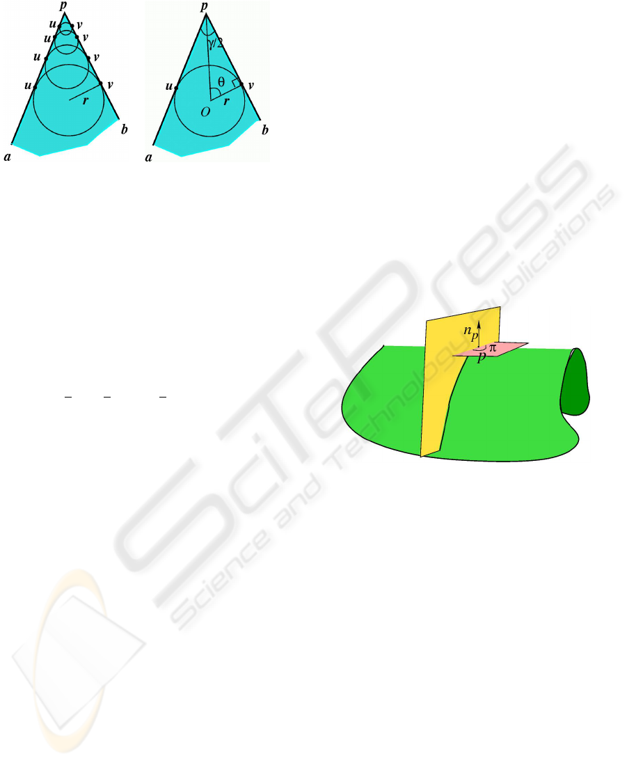
points u ∈ [p, a] and v ∈ [p, b] (see Figure 2(a)).
(a) (b)
Figure 2: In (a), circles tangent to the sector from it interior.
In (b), computing total curvature of arc (uv).
Let (uv) be the arc of S
r
delimited by u and v and
located in triangle ∆(upv). Then, the polygonal path
apb can be smoothly approximated by the path [au]∪
(uv) ∪ [vb] for any value of r (see Figure 2(a)). The
curvature value at any point of circle S
r
is constant
and equal to 1/r. Let O be the center of S
r
and θ be
the angle
d
uOp =
d
vOp. The total curvature of (uv) is
given by:
k =
Z
(uv)
1
r
dl =
1
r
l(uv) =
1
r
2rθ = π − γ. (2)
The above quantity does not depend on the radius of
circle S
r
through which we approximate the curve.
This means that π − γ is an intrinsic quantity of curve
C at vertex p since it depends only on the fracture an-
gle γ. Then, we can give the following definition:
Definition 3. Concentrated curvature of C at p is the
total curvature π −γ of arcs (uv) approximating curve
C around point p. We simply call it Ccurvature and
we denote it by k
C
(p).
Let C be a discrete piecewise-linear oriented pla-
nar curve. Suppose that C is parameterized, and hence
oriented, by its natural arc length s and that the posi-
tive angle orientation is counterclockwise. At a vertex
of the curve for which the next segment is not aligned
with the previous one, the deviation angle γ at the ver-
tex is computed in the positive sense from the pre-
vious segment to the new segment. With this con-
vention the Ccurvature π − γ of a parameterized curve
may have negative or positive values.
4 CCURVATURE FOR
TRIANGULATED 3D SURFACES
Let Σ be a piecewise linear triangulated surface and
p be a vertex of Σ. Let
−→
n be the normal vector at p
defined by the average of the normal vectors of the
triangles incident in p. Let Π be a plane passing by p
and containing the normal vector
−→
n . This plane cuts
surface Σ along a polygonal curve C = Σ ∩ Π con-
taining point p. We compute the Ccurvature k
C
(p) at
point p of curve C as described in Section 3. Note
that the position of the normal vector
−→
n with respect
to the polygonal curve C should be taken into account.
If the normal vector
−→
n and the polygonal curve C
lie in two different half planes (or equivalently they
are separated by the “tangent” plane T
p
whose normal
vector is
−→
n , see Figure 3), then the angle γ of C at
p is smaller than π and the Ccurvature value π − γ is
positive. Otherwise, the angle γ of C at p is larger
than π and the Ccurvature value π − γ is negative. In
this case, for simplicity of computation, we observe
that if γ
0
is the geometric angle of C at p (i.e., γ
0
is the
supplementary angle of γ: γ + γ
0
= 2π), then we have
π − γ = γ
0
− π. This Ccurvature value corresponds to
the normal curvature at vertex p.
Figure 3: Intersection of plane Π with a smooth surface.
Angle at p is divided into two equal angles.
When plane Π turns around
−→
n , we obtain a set of
Ccurvature values bounded (respectively from below
and from above) by two extremal values k
C,1
(p) ≤
k
C,2
(p) . Values k
C,1
(p) and k
C,2
(p) correspond to the
principal curvatures. Based on them, we can define
a mean and a Gaussian curvature, in a similar way as
we do in the analytic case:
Definition 4. The extremal values k
C,1
(p) and k
C,2
(p)
bounding the set of k
C
(p)’s are called the principal
Ccurvatures at vertex p.
Definition 5. The Gaussian Ccurvature K
C1
(p) of Σ
at vertex p is defined as the product k
C,1
(p) ∗ k
C,2
(p).
Definition 6. The mean Ccurvature H
C
(p) of surface
Σ at vertex p is defined as the mean value of all nor-
mal Ccurvature values obtained by turning plane Π
around the normal vector.
Note that all these values are intrinsic values de-
pending only on the local geometric shape of surface
Σ.
GRAPP 2010 - International Conference on Computer Graphics Theory and Applications
92
In practice, we cannot compute all the normal
Ccurvature values (k
C
(p)) since the rotation of plane
Π generates an infinite sequence of values. We can
extract a subsequence for computing an approxima-
tion of principal Ccurvatures.
Following the way in which normal curvature is
defined for smooth surfaces (see Section 2), we simu-
late a discrete rotation around the normal vector
−→
n
p
at
a vertex p of the plane Π containing
−→
n
p
, by consider-
ing one plane for each vertex v
i
in the star of p. Given
v
i
, we take the curve where plane Π
i
, containing p,
−→
n
p
and v
i
, intersects the star of p, and compute its cur-
vature. This process gives a discrete rotation around
p. Each intersection curve is a polygonal line (v
i
pw
i
)
where w
i
is the intersection point between plane Π
i
and the link of p. The angle γ
i
= [v
i
pw
i
, in the interior
of the cone, between vectors
−→
pv
i
and
−→
pw
i
is defined by
γ
i
:= arccos(
<
−→
pv
i
,
−→
pw
i
>
pv
i
.pw
i
). The normal Ccurvature at p
of the polygonal line (v
i
pw
i
) is defined by ∓(π − γ
i
).
The sign +1 or −1 is defined by following the po-
sition of the normal vector
−→
n
p
with respect to the
polygonal line (v
i
pw
i
) as explained above. Follow-
ing this construction, principal, mean and Gaussian
Ccurvatures can be defined at p.
5 EXPERIMENTAL RESULTS
In this Section, we experimentally compare our
Ccurvatures with other classic approaches to compute
discrete curvatures.
We compare Gaussian Ccurvature with concen-
trated curvature (described in Section 2) and with
Gaussian angle deficit. The Gaussian angle-deficit
curvature estimator (Meyer et al., 2003) is defined at
a vertex p by
K
p
=
1
A
(2π − Θ
p
), (3)
where Θ
j
is the angle at p formed by the j-th triangle
incident at p, and A is the area of the 1-ring neighbor-
hood around p or the Voronoi region around p.
We compare mean Ccurvature with mean angle
deficit. The mean angle-deficit curvature estimator
(Meyer et al., 2003) is defined, at point p, as the mag-
nitude of the following mean curvature vector nor-
malized by the area of the surrounding (Voronoi or
barycentric) neighborhood:
H
p
=
1
4
N
∑
j=1
(cotα
j
+ cot β
j
)(p − x
j
), (4)
where angles α
j
and β
j
correspond to the remaining
summits of the quadrilateral formed by the two trian-
gles adjacent to edge px
j
. Sign ± is assigned to |H
p
|
following the direction of the mean curvature vector
with respect to the normal vector of the surface at
point p.
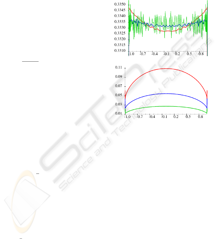
5.1 Behavior on the Sphere
Mean angle deficit
Mean Ccurvature
Figure 4: Curvature values along a meridian of the sphere,
approximated with a polyhedron made up of 5k (red), 20k
(blue), 80k (green) triangles.
The objective of discrete curvature estimators is
not to produce discrete curvature values close to an-
alytic ones, but to exhibit the same behavior as the
analytic ones, although they may produce curvature
values in their own range. This is sufficient for many
applications (e.g., mesh segmentation at lines of min-
imal curvature).
On a sphere, both Gaussian and mean analytic
curvatures are constant. Since discrete curvature es-
timators are mesh-dependent, we analyze their be-
havior on different triangle meshes approximating the
sphere. If a sphere is approximated by a regular poly-
hedron (e.g., an icosahedron), then all discrete estima-
tors give the same value at all vertices, as expected.
Another way to approximate a sphere is drawing a
number of tracks and sectors and triangulating the re-
sulting net (the resolution is controlled by varying the
number of tracks and sectors). Here, not all trian-
gles and angles are equal, and thus the discrete es-
timators give variable results. We performed our tests
with triangle meshes at increasing resolutions. Fig-
A GEOMETRIC APPROACH TO CURVATURE ESTIMATION ON TRIANGULATED 3D SHAPES
93
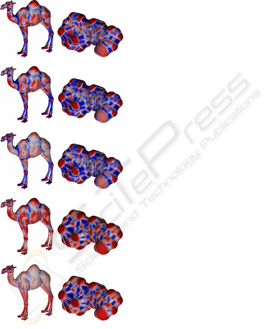
Gaussian Ccurvature
Concentrated curvature
Gaussian angle deficit
Mean Ccurvature
Mean angle deficit
Figure 5: The various curvatures on the Camel and the
Retinal meshes, in color scale.
ure 4 shows the curvature values along a meridian
of the sphere, at various resolutions, for mean angle
deficit and mean Ccurvature. Gaussian Ccurvature
and concentrated curvature are very close, and sim-
ilar to mean Ccurvature. Gaussian curvature behaves
in a similar way as mean angle deficit. All estimators
are affected by the different shape and size of trian-
gles at the various latitudes, and give abnormal values
at poles. Unlike all others, the two angle deficit mea-
sures provide higher values near the poles than near
the equator of the sphere. Angle deficit estimators
show a relevant noise, which becomes worse while
increasing resolution, because of the division by area.
The values of other measures vary smoothly along
latitude, and tend to be closer to a constant value at
higher resolutions.
5.2 Comparisons on Discrete 3D Shapes
We compare the curvature estimators on triangulated
shapes of different kinds from the AIM@SHAPE
repository (http://shapes.aim-at-shape.net/). The
Camel mesh has 9770 vertices and 19536 triangles;
the Retinal molecule mesh has 3643 vertices and 7282
triangles. Curvature values are plotted in a color scale
in Figure 5. The color scale is from blue (minimum
negative value) through white (zero) to red (maximum
positive value), where the minimum and maximum
values may be different in the specific curvature esti-
mators.
Gaussian Ccurvature and concentrated curvature
have a very similar behavior. The two angle deficit
measures tend to give near-zero values (white) to
wider areas, while the other estimators better follow
the geometrical shape of the surface. This is espe-
cially evident on Camel mesh. On Retinal molecule,
all mean estimators and all Gaussian estimators be-
have similarly. The mean and Gaussian Ccurvature
values seem to provide a slightly better delimitation
of positive and negative curvature areas.
In estimating Ccurvatures, we approximate the
continuous rotation of the plane around the surface
normal at a vertex p, in a discrete way, by using just
the planes passing through the neighbors of p. To
get more precision, we may refine the link (i.e., the
boundary of the star) of p by adding new points on
its edges, and consider a plane through each of them.
Experiments show the resulting (mean and Gaussian)
Ccurvature values are almost the same, and this con-
firm the validity of the approach.
To illustrate the application of curvature to 3D
shape segmentation, we show in Figure 6 two seg-
mentations based on mean Ccurvature, which high-
light convex features.
GRAPP 2010 - International Conference on Computer Graphics Theory and Applications
94

Figure 6: Segmentations of 3D shapes based on mean
Ccurvature.
6 CONCLUDING REMARKS
We have presented a geometrical technique to esti-
mate discretely normal, principal, mean and Gaus-
sian curvatures on a triangulated piecewise linear sur-
face. Our technique describes well the local geo-
metric shape of the surface. The experimental re-
sults we presented validate the approach and show
that Ccurvature behaves better than some mostly used
techniques.
It would be interesting to further investigate the
stability, or convergence of Ccurvature values to some
intrinsic value, when adding more points to refine the
discrete rotation of the cutting plane around a vertex
normal.
Concentrated curvature of polygonal curves has
interesting applications for spatial curves to charac-
terize them via an additional discrete torsion notion,
this will leads to interesting applications in GPS field
and robotics (3D motion for example).
The principle of concentrated curvature has also
been used to define discrete estimators for scalar cur-
vature of 3-combinatorial manifolds.
ACKNOWLEDGEMENTS
This work has been partially supported by the Na-
tional Science Foundation under grant CCF-0541032.
REFERENCES
Akleman, E. and Chen, J. (2006). Practical polygonal mesh
modeling with discrete gaussian-bonnet theorem. In
Proceedings of Geometry, Modeling and Processing.
Alboul, L., Echeverria, G., and Rodrigues, M. A. (2005).
Discrete curvatures and gauss maps for polyhedral
surfaces. In Workshop on Computational Geometry.
the Netherlands.
Aleksandrov, P. (1957). Topologia combinatoria. Torino.
Borrelli, V., Cazals, F., and Morvan, J.-M. (2003). On
the angular defect of triangulations and the pointwise
approximation of curvatures. Comput. Aided Geom.
Des., 20(6):319–341.
Do Carno, M. P. (1976). Differential Geometry of Curves
and Surfaces. Prentice-Hall, Inc.
Doss-Bachelet, C., Franc¸oise, J.-P., and Piquet, C. (2000).
G
´
eom
´
etrie diff
´
erentielle. Ellipses.
Gatzke, T. and Grimm, C. (2006). Estimating curvature
on triangular meshes. International Journal of Shape
Modeling, 12(1):1–29.
Hahmann, S., Belyaev, A., Bus
´
e, L., Elber, G., Mourrain,
B., and Roessl, C. (2007). Shape Interrogation. In
Shape Analysis and Structuring, Mathematics and Vi-
sualization, pages 1–57. Springer.
Meyer, M., Desbrun, M., Schr
¨
oder, P., and Barr, A. H.
(2003). Discrete differential-geometry operators for
triangulated 2-manifolds. In Visualization and Mathe-
matics III, pages 35–57. Springer-Verlag, Heidelberg.
Surazhsky, T., Magid, E., Soldea, O., Elber, G., and Rivlin,
E. (2003). A comparison of gaussian and mean cur-
vatures estimation methods on triangular meshes. In
Proceedings of Conference on Robotics and Automa-
tion, 2003., pages 739–743.
Taubin, G. (1995). Estimating the tensor of curvature of
a surface from a polyhedral approximation. In ICCV
’95: Proceedings of the Fifth International Confer-
ence on Computer Vision, page 902.
Troyanov, M. (1986). Les surfaces euclidiennes singularits
coniques. Enseign. Math. (2), 32:79–94.
Watanabe, K. and Belyaev, A. G. (2001). Detection of
salient curvature features on polygonal surfaces. Com-
put. Graph. Forum, 20(3):385–392.
Xu, G. (2006). Convergence analysis of a discretization
scheme for gaussian curvature over triangular sur-
faces. Comput. Aided Geom. Des., 23(2):193–207.
A GEOMETRIC APPROACH TO CURVATURE ESTIMATION ON TRIANGULATED 3D SHAPES
95
