APPARENT MOTION ESTIMATION USING PLANAR
CONTOURS AND FOURIER DESCRIPTORS
Fatma Chaker and Faouzi Ghorbel
Ecole Nationale des Sciences de l’Informatique, Campus Universitaire La Manouba, Tunis, Tunisie
Keywords: Affine Arc Length, Affine Transformation, Apparent Motion, Fourier Descriptors, Parameterization.
Abstract: In the present paper, we present a Fourier-based method for global apparent motion estimation. We apply
this method for the estimation of the 2D affine transform linking two planar and closed curves. The
originality of the method relies on the estimation of the parameters not in the original space but in the
transformed space: Fourier space. This technique does not require explicit point to point correspondences;
in fact such point correspondences are a by-product of the proposed algorithm. Experimental results and
applications validate the use of our technique.
1 INTRODUCTION
Parametric model motion estimation can be used in
many computer vision applications such object-
based video coding, content-based video
manipulation or video indexing and retrieval by
content.
Accurate correspondences are needed in most
algorithms which compute algebraic relationships.
Generally, they use features or primitives ranging
from simple points to complex ones like conics
(Kruger, 1998) (Kantani, 1996) (Sugimoto, 2000)(
Kumar, 2004) ( Hartley, 2004) (Kumar, 2006).
Assumptions on the imaging setup are also made.
An affine motion model is often adopted because it
can describe many real motions. For example, a
plane in general 3D motion under orthographic
projection, an object translating at a constant depth,
etc.
In this paper, we present a novel Fourier domain
technique to compute the apparent affine motion
between two views that only needs corresponding
contours - no explicit point-to point correspondence
is needed. In fact, the point-to-point correspondence
is obtained as a by-product of our affine motion
computation scheme.
Apparent motion estimation has been estimated
using many geometrical primitives. A detailed
review and relative performance comparisons may
be seen in (Agarwal, 2005).
The proposed technique was inspired from the
research of (Ghorbel, 1996). In this work, a motion
estimation algorithm based on FDs was developed in
the case of similarity group (translation, rotation and
zoom).
The algorithm proposed in this paper, in addition
to similarity group parameters, allows the estimation
of stretching ones. Under stretching, the shape of the
object will no longer be preserved. Such shape
distortion can typically arise if a planar object is
observed by a camera under arbitrary orientation
with respect to the plane. The relative positions of
the camera and the objects are arbitrary, but the
viewing conditions are supposed to be such that
orthogonal projection combined with a scaling factor
allows a good approximation of the perspective
projection.
Under these conditions, two views of the
contours of the same object are known to be related
to each other by a two-dimensional affine
transformation (Pauwels, 1995). These
transformations constitute the special affine motion
group SA(2).
The rest of the paper is organized as follows:
In Section 2, we describe the used
parameterization and description procedures. The
apparent affine motion algorithm based on FDs is
presented in Section 3. Section 4 is dedicated to the
algorithm evaluation using a synthetic and real data.
322
Chaker F. and Ghorbel F. (2010).
APPARENT MOTION ESTIMATION USING PLANAR CONTOURS AND FOURIER DESCRIPTORS.
In Proceedings of the International Conference on Computer Vision Theory and Applications, pages 322-327
DOI: 10.5220/0002826603220327
Copyright
c
 SciTePress

2 PARAMETERIZATION,
NORMALIZATION,
DESCRIPTION
2.1 Parameterization
Different parameterizations can be used to represent
a given curve. The normalized arc length l is
required when considering invariance under
similarities. It is the same for the estimation of the
global movement of objects assumed to be rigid.
Pointwise correspondence between two equivalent
curves can then be achieved efficiently.
In the case of affine motion group the re
parameterization can be formulated in terms of the
action of affine motion group SA(2).
The special affine motion group SA(2) can be
seen as the product of R
2
SL(2) where SL(2) is the
special plan linear transformations group. The
choice of the suitable parameterization implies that
the action of the affine motion group SA(2) can be
described by the following operation:









 B,
0
llαAXX,α,
0
lA,B,
,
1
S
2
2
R
L
1
S
2
2
R
1
S2SL
2
R


R
L
(1)
where S
1
is the unit circle of the plane R
2
, l
0
the
shift, A is the affine matrix with the determinant of
A such that Det(A)=1 and X is a parameterization of
an object O.
The reparametrization-invariance is a crucial
problem. In deed, when comparing different views
of a planar contour we cannot assume that the
parameterizations are the same. To avoid this
problem we must ensure that the expressions for the
motion affine parameters are independent of the
choice of parameterization.
In the case of motion affine group, it is well
known that from any object O we can extract a
periodic normalized affine arc length
parameterization (Spivac, 1970).
In our case we have used the periodic normalized
affine arc length function l(t) defined by :
  



t
a
,duuX,u'Xdet
L
tl
0
3
1
 



Tt
a
,duuX,u'XdetL
0
3
(2)
Where X’ and X” denote, respectively, first and
second derivatives of X, while
det represents the de-
terminant operator.
In order to describe the affine parameters we
have to define the relationship between two curves
having the same shape, in terms of corresponding
normalized affine arc length parameterizations.
The closed contour X
2
will be said to be similar
to the closed contour X
1
, if X
2
can be mapped into
X
1
by a composition of affine transformation A, a
translation
B, and a scale change .
In terms of normalized affine arc length
parameterization, we say that two objects
O
1
and O
2
have the same affine shape if and only if:




,llXlX BA 



012
(3)
where X
2
and X
1
are, respectively, a normalized
affine arc length parameterization of
O
2
and O
1
, A is
an element of SL(2) and
B is a vector of R
2
.
2.2 Fourier Descriptors
The Fourier descriptors (FDs) are a set of
coefficients of the Fourier transform derived from
the outline of an object and which has been used in
widely pattern recognition applications. It has been
proved that most of the information about the shape
is contained in the first few (lower frequency)
coefficients, and that noise usually affects only the
details of the shape and consequently only the higher
frequency coefficients of the FDs. Therefore, pattern
recognition is carried out by examining only the first
few coefficients.
The following lemma gives the relationship
between Fourier coefficients of X
1
and X
2
.
Lemma (Shift theorem). Let X
1
and X
2
be,
respectively, the normalized affine arc length
parameterizations of two objects having the same
affine-shape. Then for all integer k,


k
jkl
kek 

BA
1
2
2
UU
0
(4)
where U
1
(k) and U
2
(k) are respectively the bi-
dimensional complex vectors formed by the Fourier
coefficients of components of X
1
and X
2
, while :





otherwise
Mkif
k
0
1
is the Kronecker symbol, M is the normalized
number of points contour.
The translation vector
B corresponds to the DC
component (k= 0) in the frequency domain. It can be
neglected initially by shifting the origin to the
centroid of the contour. Later,
B can be trivially
computed as the difference in the centroid of the two
APPARENT MOTION ESTIMATION USING PLANAR CONTOURS AND FOURIER DESCRIPTORS
323

sequences.
Since
A is a linear transformation, it can be
shown that same transformation (
A) relates the
sequences in both the spatial as well as frequency
domains (Ghorbel, 1996), (Ghorbel, 1998),
(Kuthirummal, 2002). The action on the Fourier
space is reduced to the following operation:


  ).k(Ue,l,
*),Z(L*)Z(LRS)(SL
jkl
RR
AA
0
22
0
221
2


(5)
3 APPARENT AFFINE MOTION
ESTIMATION
In the following we will present the different steps
used in our algorithm to estimate the parameters of
the affine apparent motion.
3.1 Determination of Scaling ()
By taking the determinant of the 22 matrices
defined by the vectors
))(),((
*
kUkU
h
h
and
))(),((
*
kUkU
f
f
on some fixed index k, we have the
following equality:
))(),(det())(),(det(
*2*
kUkUkUkU
f
f
h
h
 
(6)
Therefore the scaling is:




 

kU,kU
kU,kU
*
f
f
*
h
h
det
det
2

(7)
Where U* is the complex conjugate of U.
3.2 Determination of Shift l
0
Taking the determinants of the matrices






211
k
f
,Uk
f
UM 



212
kU,kUM
hh

and
we obtain :
)1(det)(det)(det
021
)(
2
2
MeM
lkkj
A

 
where k
1
and k
2
two fixed indices.
Taking the argument of this expression:
))M((l)kk())M((
10212
detargdetarg 
We then obtain:




21
12
0
MdetargMdetarg
kk
l



(8)
Where arg(Z) is the complex argument of U.
3.3 Computation of
Parameters Matrix A
Let us assume that the scale end shift values are
determined by (7) and (8), respectively. In this
section we would like to compute the parameters of
the matrix
A. In the following we will use the vector
representations:

















































kv
ku
kU;
kv
ku
kU
;
ky
kx
kX;
ky
kx
kX
hf
2
2
1
1
2
2
2
1
1
1
(9)
where u
i
and v
i
are, respectively, the Fourier
descriptors of x
i
and y
i
(i=1,2).
Using the shift theorem, we have:
 
kUekU
f
jkl
h
A
0

(10)
Substituting Equation 9 in 10 gives for all k  M:




























kv
ku
aa
aa
e
kv
ku
jkl
1
1
43
21
2
2
0
(11)
The extraction of apparent motion consists on
extracting the parameters of the matrix
A from the
following equations set:














)k(AUe)k(U
.
.
.
)k(AUe)k(U
)k(AUe)k(U
nf
jkl
nh
f
jkl
h
f
jkl
h
0
0
0
22
11
(12)
This system of 2N equations and 2 unknown can
be written as:
VISAPP 2010 - International Conference on Computer Vision Theory and Applications
324
















)k(vae)k(uae)k(v
)k(vae)k(uae)k(u
.
.
.
)k(vae)k(uae)k(v
)k(vae)k(uae)k(u
nn
jkl
nn
jkl
n
nn
jkl
nn
jkl
nn
jkljkl
jkljkl
431
21
11411312
11211112
00
00
00
00
(13)
which can be written as:
nn
UK
242

 4
A
(14)
and more precisely:

















































)(
)(
.
.
.
)(
)(
)()(00
00)()(
.
.
)()(00
00)()(
2
2
12
12
4
3
2
1
11
11
1111
1111
00
00
0101
0101
n
n
n
ljk
n
ljk
n
ljk
n
ljk
ljkljk
ljkljk
kv
ku
kv
ku
a
a
a
a
kvekue
kvekue
kvekue
kvekue
nn
nn
(15)
This is a linear system of equations with 2N
equations and four unknowns (elements of A). It can
be solved for A. The resolution of the system
defined by (14) is obtained by:

UKKK
tt
1


4
A
(16)
In deed, the equation (14) can be written as follows:
eUK A
(17)
e represents the error vector. The best solution
(A) is that which minimize the module of the error
vector. We search, hence, A for which
eee
t

2
is
minimum. This consists on minimizing the system
using the pseudo inverse of K.
4 RESULTS AND DISCUSSIONS
In this section, we present the results from a number
of experiments conducted to affirm the validity of
the algorithm presented in the previous section.
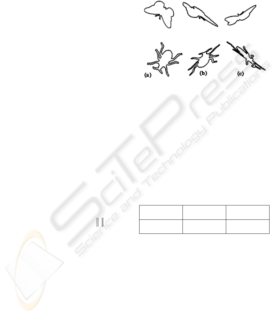
For the first experiment, we use the planar
boundary of images “Butterfly” and “Insect” in a
reference view for the study. Other views were
generated using affine transformations to map points
in the reference view into the new views (Figure 2).
The figure is arranged as follows. In part (a) we list
the input contours. Parts (b) and (c) illustrate the
contours obtained by applying the considered affine
transformation.
The shape boundaries in the views were sampled
so that each shape was represented by 1024 points.
Figure 1: Two affine transformed views of contours
“Butterfly” and “Insect”.
These contours are used as input to our algorithm
and we estimate the affine transformation. The re-
projection error (error between the actual second
contour and the warped contour generated by
applying the estimated affine transformation over
the initial contour) is very low as shown in Table 1.
Table 1: Values of the re-projection error. The first
column present the values of the re-projection error
between the actual second contours ((b) in Figure 1) and
the warped contour generated by the estimated affine
transformation. The second column present the values of
the re-projection error between the actual second contours
(c) and the warped contour generated by the estimated
affine transformation.
Butterfly
0.05149 0.00620
Insect
0.016545 0.004086
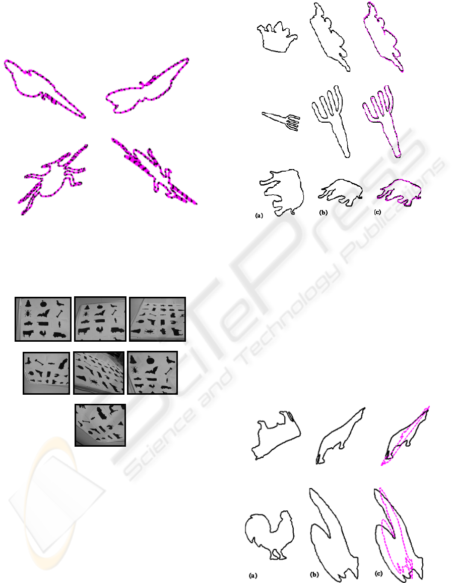
Figure 2 shows the overlay of contours (a)
transformed by the estimated affine transformation
over contours (b) and (c).
In the second experiment we consider a variety
of images from various situations in real-life. These
images are used to demonstrate the effectiveness of
our algorithm in a variety of real-life situations. The
Multiview Curve Dataset (MCD) (Zuliani, 2004)
was used to carry out this experiment. This dataset
comprises 40 shape categories, each corresponding
to a shape drawn from an MPEG-7 shape category.
Each category in the new dataset contains 7 curve
samples that correspond to different perspective
distortions of the original shape. The original
MPEG-7 shapes were printed on white paper and 7
APPARENT MOTION ESTIMATION USING PLANAR CONTOURS AND FOURIER DESCRIPTORS
325

samples were taken using a digital camera from
various angles (Figure 1). The contours were
extracted from the iso-intensity level set
decomposition of the images (Lisani, 2001).
Figure 2: Overlay of first “Butterfly” and “Insect”
contours ((a) in Figure 2) wrapped over second contours
((b) and (c) in Figure 2) by the estimated affine
transformation. The magenta colored dash-dotted line is
the warped contour and black colored dotted line is the
actual contour.
(a) (b) (c)
(d) (e) (f)
(g)
Figure 3: Some Examples of Images from the MCD
database acquired from different viewpoints; (a): Central
(b) Bottom (c) Left (d) Right, (e) Top (f) Top-left, (g)
Bottom- Right.
Figure 4 shows same results obtained from the
MCD dataset. The figure is arranged as follows. In
parts (a) and (b) we list the input contours, (c) shows
the overlay of contour (a) transformed by estimated
transformation over (b). The high overlap between
the contours clearly shows the correctness of our
algorithm. This experiment shows that the given
algorithm produce the correct affine transformation
for a variety of situations. This makes the algorithm
acceptable for various real-life situations.
Figure 4: (a), (b) input contours extracted from images
taken from different point of view. (c) Overlay of contour
(b) with (a) warped by the estimated affine transformation.
Strong distortions show some errors in the
estimate and some examples of such contours are
shown in Figure 5. The contours are highly distorted
and it is difficult for even a human to identify the
contours. The figure is arranged as follows. In part
(b) we present highly deformed images of contours
(a). Part (c) shows the overlay of first contours (a)
wrapped over second contours (b) by the estimated
affine transformation. The magenta colored dash-
dotted line is the warped contour and black colored
dotted line is the actual contour.
Figure 5: Examples of failure cases of the proposed
algorithm.
VISAPP 2010 - International Conference on Computer Vision Theory and Applications
326

5 CONCLUSIONS AND FUTURE
WORK
In this paper we have presented a novel Fourier
domain technique to estimate the affine apparent
motion between two views that only needs
corresponding contours. Our technique does not
need explicit point-to-point correspondence. The
normalization of the contours based on the affine arc
length was indispensable when the movement is
assumed affine.
Experiments have shown the applicability of our
technique to a variety of real world problems.
In a future work we would extend our method for
projective homography estimation.
Further experiments would be carried out to
validate our experiments. Parameters such as the
number of points, noise (discretization, sampling,
localization etc.), symmetry in contour, occlusion,
etc. can affect the performance of the proposed
algorithm. An analysis with respect to these
parameters can prove further the performance of the
proposed technique.
REFERENCES
Agarwal, A., Jawahar, C. V. and Narayanan, P. J. A
Survey of Planar Homography Estimation Techniques.
IIIT Technical Report IIIT/TR/2005/12, June 2005.
Ghorbel, F., Mokadem, A., Daoudi, M., Avaro, O. and
Sanson, H. Global planar rigid motion estimation
applied to object-oriented coding, Conf. Proc. ICPR
96, vol. I, 1996, pp. 641-645.
Ghorbel. F. Towards a unitary formulation for invariant
images description: application to images coding,
Annales des Télécommunications, France 1998.
Hartley, R.I. and Zisserman, A. Multiple View Geometry
inComputer Vision, 2nd Edition. Cambridge
University Press, 2004.
Kanatani, K. Statistical Optimization for Geometric
Computation: Theory and Practice. Elsevier Science,
1996.
Kruger, S. and Calway, A. Image Registration Using
Multiresolution Frequency Domain Correlation. In
British Machine Vision Conference (BMVC), pages
316.325, September 1998.
Kumar, M. P., Goyal, S., Kuthirummal, S., Jawahar, C. V.
and Narayanan, P. J. Discrete Contours in Multiple
Views: Approximation and Recognition. Journal of
Image and Vision Computing (IVC),
22(14):1229.1239, December 2004.
Kumar, M. P., Jawahar, C. V. and Narayanan, P. J.
Geometric Structure Computation from Conics. In
Proceedings of Indian Conference on Computer
Vision, Graphics, and Image Processing (ICVGIP),
pages 9.14, 2004.
Kumar, P. J., Jawahar, C. V. "Homography Estimation
from Planar Contours," 3dpvt, pp.877-884, Third
International Symposium on 3D Data Processing,
Visualization, and Transmission (3DPVT'06), 2006.
Kuthirummal, S., Jawahar, C. V. and Narayanan, P. J.
Planar Shape Recognition across Multiple Views. In
Proceedings of the International Conference on
Pattern Recognition (ICPR), pages 482.488, August
2002.
Lisani, J. L. Shape based Automatic Images Comparison,
Ph.D. Thesis, University Paris IX-Dauphine, 2001.
Pauwels, E. J., Recognition of planar shapes under affine
distortion, Int. J. Comput. Vision 14(1995) 49-65.
Sugimoto, A., A Linear Algorithm for Computing the
Homography from Conics in Correspondence. Journal
of Mathematical Imaging and Vision, 13:115.130,
2000.
Zuliani, M., Bhagavathy, S., Manjunath, B. S. and
Kenney, C. S. Affine-Invariant Curve matching. 2004.
APPARENT MOTION ESTIMATION USING PLANAR CONTOURS AND FOURIER DESCRIPTORS
327