GPU OPTIMIZER: A 3D RECONSTRUCTION ON THE GPU USING

MONTE CARLO SIMULATIONS

How to Get Real Time without Sacriﬁcing Precision

Jairo R. S

anchez, Hugo

Alvarez and Diego Borro

CEIT and Tecnun (University of Navarra) Manuel de Lardiz

abal 15, 20018 San Sebasti

an, Spain

Keywords:

3D reconstruction, Structure from motion, SLAM, GPGPU.

Abstract:

The reconstruction of a 3D map is the key point of any SLAM algorithm. Traditionally these maps are built

using non-linear minimization techniques, which need a lot of computational resources. In this paper we

present a highly paralellizable stochastic approach that ﬁts very well on the graphics hardware. It can achieve

the same precision as non-linear optimization methods without loosing the real time performance. Results are

compared against the well known Levenberg-Marquardt algorithm using real video sequences.

1 INTRODUCTION

Real time simultaneous localisation and mapping

(SLAM) consists of calculating both the camera

motion and the 3D reconstruction of the observed

scene at the same time. This work addresses the 3D

reconstruction problem, i.e., obtaining a set of 3D

points that represents the observed scene using only

the information provided by a single camera.

If the required precision is high, existing re-

construction algorithms are usually very slow and

not suitable for real time operation. This work

proposes an implementation that can achieve a high

level of accuracy in real time, taking advantage of the

graphics hardware available in any desktop computer.

This work develops a new 3D reconstruction algo-

rithm based on Monte Carlo simulations that can be

directly executed on a modern GPU. The algorithm

consists of approximating the maximum likelihood

estimator, random sampling from the space of pos-

sible locations of the 3D points. Since each sample

is independent from others, this method exploits well

the data level parallelism required by this program-

ming model.

For validating it, we have compared both preci-

sion and performance with the implementation of the

Levenberg-Marquardt non-linear minimization algo-

rithm given in (Lourakis, 2004).

2 PROBLEM DESCRIPTION

It is assumed that there is an image source that feeds

the algorithm with a constant ﬂow of images. Let

be the image of the frame k. Each image has a

set of features associated to it given by a 2D feature

tracker Y



,...,~y



. Feature ~y

has





coordinates. The 3D motion tracker calculates the

camera motion for each frame as a rotation matrix and

a translation vector x





, where the set of all

computed cameras up to frame t is X

{

,...,x

}

The problem consists of estimating a set of 3D points

{

,...,~z

}

that satisﬁes the following equation:

= Π





∀i ≤ n, ∀k ≤ t (1)

where Π is the pinhole projection function. For

simplicity, the calibration matrix can be obviated in

Equation 1 if 2D feature points are represented in

normalized coordinates instead of pixel coordinates.

2.1 Proposed Algorithm

A 3D structure optimization method is proposed, that

performs a global minimization using a probabilisti-

cal approach based on the Monte Carlo simulation

paradigm (Metropolis and Ulam, 1949). This ap-

proach consists of generating inputs randomly from

the domain of the problem. These possible solu-

tions are then weighted using some type of function

depending on the measurement obtained from the

system. Monte Carlo simulations are suitable for

443

R. Sánchez J., Álvarez H. and Borro D. (2010).

GPU OPTIMIZER: A 3D RECONSTRUCTION ON THE GPU USING MONTE CARLO SIMULATIONS - How to Get Real Time without Sacriﬁcing

Precision.

In Proceedings of the International Conference on Computer Vision Theory and Applications, pages 443-446

DOI: 10.5220/0002826704430446

 SciTePress

problems were it is not possible to calculate the exact

solution from a deterministic algorithm, i.e., the case

of 3D reconstruction from 2D image features, since

the direct method is ill-conditioned.

However, this strategy leads to very computation-

ally intensive implementations that makes it unusable

for real time operation. One of the key features

of these simulations is that each possible solution

is computed independently from others, making it

optimal for data-streaming architectures, like GPUs.

This system completments the 3D camera tracker

presented in (Eskudero et al., 2009) that also runs on

the GPU using a similar paradigm.

Every new frame, at time t + 1, the set Z

enlarged with new points and reﬁned with the new

observations Y

t+1

provided by the feature tracker,

getting a new set Z

t+1

. Unlike probabilistic batch

methods, the proposed optimizer uses all the available

frames for doing this optimization, since the GPU can

handle them comfortably. Of course, there is a limit

in the amount of frames that the GPU can process in

real time. The overall view of the proposed method

has the following steps:

1. Initialize New 3D points. The algorithm tries to

triangulate new 3D points using the feature points

provided by the tracker.

2. Generate Samples from Nnoisy 3D Points. The

system generates new hypotheses about the lo-

cation of the 3D points using the available 3D

structure as initial guess.

3. Evaluate the Hypotheses. Hypotheses are evalu-

ated using an objective function that computes the

projection residual of all the samples against all

the available measurements. The best one is used

as new location for the 3D point.

3 GPU IMPLEMENTATION

The algorithm is composed by three shader programs.

These programs will run sequentially for each point to

be optimized. The ﬁrst shader program will generate

all the hypotheses for a single point location, the sec-

ond shader program will compute the weight of each

hypothesis and the third shader program will choose

the best candidate among the hypotheses. Algorithm

1 shows a general overview of the proposed method.

The parts executed on the GPU have the GPU preﬁx.

3.1 Data Structures

Since the GPU is a hardware designed to work with

graphics, the way to load data on it, is using image

textures. The output is obtained using the render-to-

texture capabilities of the graphics card. It is very

important to choose good memory structures since

the transfers between the main memory and the GPU

memory are very slow.

In our case, the hypotheses for the location of a 3D

point are stored in a RGBA texture. Each hypothesis

has its coordinates stored in the RGB triplet and

the result of evaluating the objective function in the

alpha channel. Another similar texture is used as

framebuffer. Each texel of these textures will be a

single hypothesis, so the total number of hypotheses

for each point will be the size of the texture squared.

Another RGB texture is used for storing ran-

dom numbers generated in the CPU. This is because

graphics hardware lacks random number generating

functions. This texture is computed in preprocessing

stage and remains constant, converting this method in

a pseudo-stochastic algorithm. Interested readers can

refer to (Eskudero et al., 2009) for more details.

Algorithm 1: Overview of the GPU minimization.

for all~z

in Z

SendToGPU(~z

)

GPU SampleHypotheses()

for all ~y

{

,...,Y

}

SendToGPU(~y

, x

)

GPU EvaluateHypotheses()

end for

= GPU GetBestHypothesis()

t+1

←ReadFromGPU(

)

end for

3.2 Initialization

New points are initialized via linear triangulation.

This is a very ill-conditioned procedure and its results

are unusable, but it is a computationally cheap starting

point for the minimization algorithm. This stage is

implemented in the CPU since it runs very fast, even

when triangulating many points.

3.3 Sampling Points

In this step all the 3D points in the map are subject

to be optimized. This stage runs when new points are

triangulated and when new frames are tracked. Trian-

gulated points have large error due to ill-conditioned

systems of equations, and existing points can be

improved with the new measures provided by the

feature tracker.

VISAPP 2010 - International Conference on Computer Vision Theory and Applications

444

For each point ~z

, a set of random samples S

(1)

,...,~z

(m)

is generated around its neighborhood.

The stochastic sampling function used is a uniform

random walk around the initial point:

(n)

= f (~z

,~n

) =~z

+~n

, ~n

∼ U

(−s,s) (2)

where ~n

is a 3-dimensional uniform distribution hav-

ing minimum in -s and maximum in s. The parameter

s is chosen to be directly proportional to the prior

reprojection error of the point being sampled. In this

way, the optimization behaves adaptively avoiding

falling into local minimums and handling well points

far from the optimum. The GPU implementation is

performed using a fragment shader. The data needed

are the 3D point to be optimized and the texture

with the random numbers. The output is a texture

containing the coordinates for all hypotheses. The

only datum transfered is the 3D point coordinates,

because the the random numbers are transfered in

preprocessing stage. It is not necessary to download

the generated hypotheses to main memory, because

they are only going to be used by the shader that

evaluates the samples.

3.4 Evaluating Samples

All the set S

for every point ~z

is evaluated in

this stage. The objective function is the residual

of Equation 1 applied to every 3D point for every

available frame:

argmin

∑

k=1



( j)



−~y

(3)

Equation 3 satisﬁes the independence needed in

stream processing, since each hypothesis is indepen-

dent from others.

Hypotheses are evaluated using a different shader

program. This shader runs once for each projection

using texture ping-pong (Pharr, 2005), avoiding to

use loops inside the shader. The only data needed to

be transferred are the camera pose and the projection

of the 3D point for each frame. This shader program

must be executed t times for each 3D point.

When all the passes are rendered, the output

texture will contain the matrix with all the hypotheses

weighted. Now there are two ways to proceed. The

ﬁrst one is to download the entire texture to main

memory and then search the best candidate using the

CPU. The second one is to search directly in the GPU.

Experimentally, we concluded that the second one is

the best way if the size of the texture is big enough.

This search is performed in a parallel fashion using

reduction techniques (Pharr, 2005).

4 EXPERIMENTAL RESULTS

Both precision and performance of the proposed

method have been measured in order to validating

it. All tests are executed on a real video recorded

in 320 × 240 using a standard webcam. Results are

compared with the implementation of the Levenberg-

Marquardt algorithm given by (Lourakis, 2004). In

our setup, the GPU optimizer runs with a viewport

of 256 × 256, reaching a total of 2

hypotheses per

point. The maximum number of iterations allowed to

the Levenberg-Marquardt algorithm is 200.

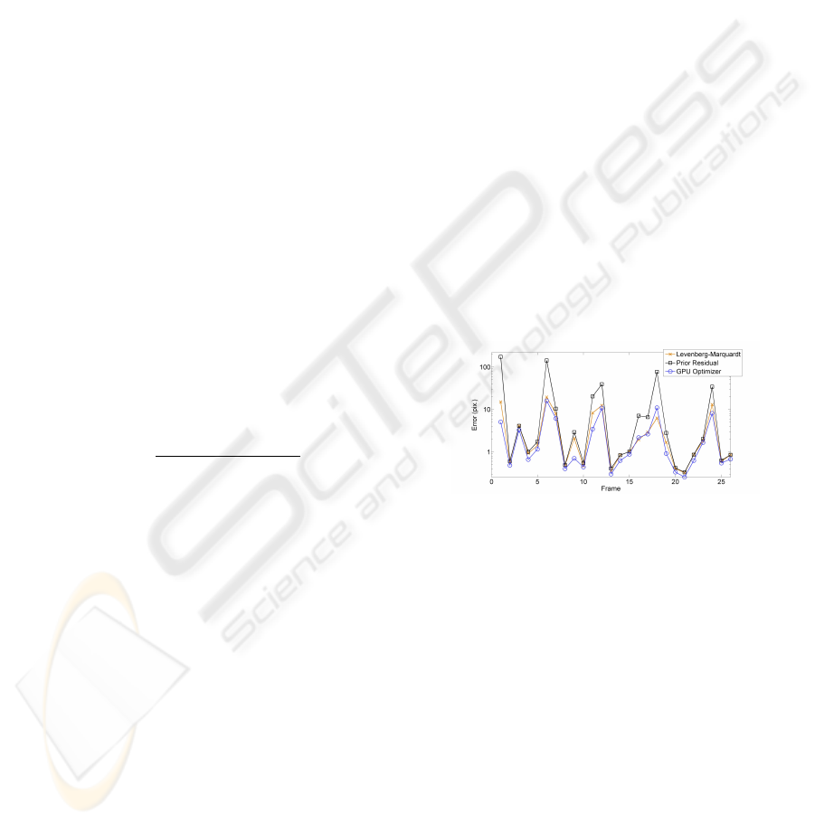
4.1 Precision

Various optimizations on triangulated 3D points have

been executed to measure the precision of the GPU

optimizer. In each run, 25 different points are re-

constructed using 15 consecutive frames tracked by

the algorithm described in (Eskudero et al., 2009).

Figure 1 shows the mean reprojection residual. The

ﬁgure is in logarithmic scale. This test shows that the

GPU optimizer gets on average 1.4 times better re-

sults than Levenberg-Marquardt, demonstrating that

both Levenberg-Marquardt and GPU optimizer get

equivalent results.

Figure 1: Residual error on real images.

4.2 Performance

The PC used for performance tests is an Intel C2D

E8400 @ 3GHz with 4GB of RAM and a nVidia

GeForce GTX 260 with 896MB of RAM memory.

Following tests show the performance comparison be-

tween the GPU optimizer and Levenberg-Marquardt.

In Figure 2, 15 points are used, incrementing in each

time step the number of frames and Figure 3 shows a

test running with 10 frames incrementing the number

of points in each time step.

Note that both ﬁgures are in logarithmic scales.

Figure 2 shows that the GPU optimizer runs ap-

proximately 30 times faster than Levenber-Marquardt

when the number of frames is increased, being capa-

ble to run at 30fps. even when optimizing 15 points

over 60 frames.

Next tests analyze deeper the time needed by the

GPU optimizer in its different phases. Figure 4 shows

GPU OPTIMIZER: A 3D RECONSTRUCTION ON THE GPU USING MONTE CARLO SIMULATIONS - How to Get

Real Time without Sacrificing Precision

445

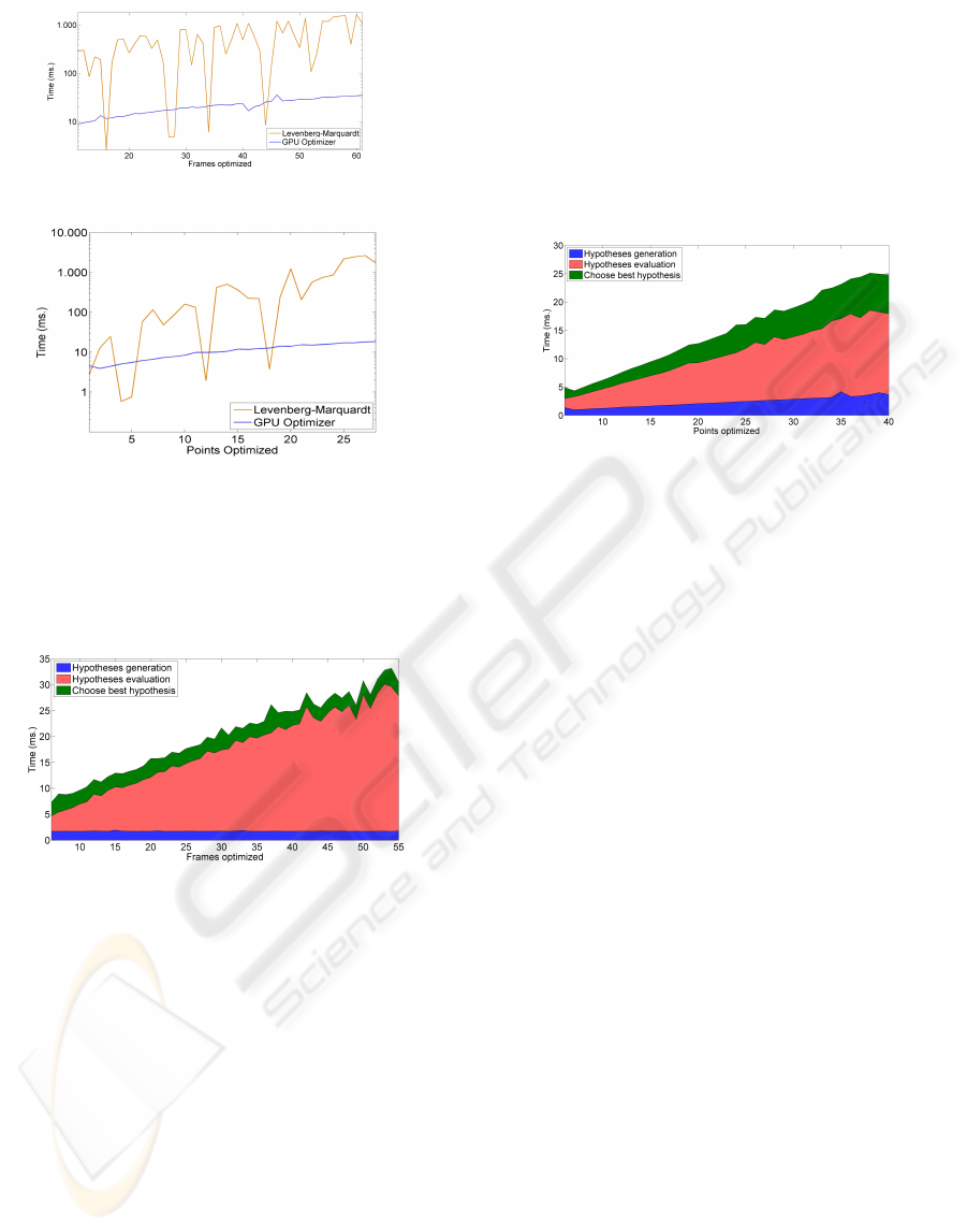
Figure 2: Performance with constant number of points.

Figure 3: Performance with constant number of frames.

the time needed to run the optimizer with 15 points

incrementing the number of frames in each time step,

and Figure 5 shows the the time needed when the

number of points to optimize is increased in each time

step, using always 10 frames.

Figure 4: Performance with constant number of points.

From Figure 4 follows that the point evaluation

is the only stage that depends on the number of

optimized frames. The total time depends linearly

on both number of points and number of frames

optimized as seen in Figure 5.

5 CONCLUSIONS

The proposed GPU optimizer runs a Monte Carlo

simulation locally on each point to be optimized,

making it very robust to outliers and highly adaptable

to different level of errors on the input data.

For validating it, a GPU implementation is

proposed and compared against the Levenberg-

Marquardt algorithm. Tests on real data show

that GPU optimizer can achieve better results than

Levenberg-Marquardt in much less time. This gain

of performance allows to use more data on the

optimization, obtaining better precision without

loosing the real time operation. Moreover, the GPU

implementation leaves the CPU free of computational

charge so it can dedicate its time to do other tasks. In

addition, the tests have been done in a standard PC

conﬁguration using a standard webcam, making the

method suitable for middle-end hardware.

Figure 5: Performance with constant number of frames.

ACKNOWLEDGEMENTS

The contract of Jairo R. S

anchez is funded by the

Ministry of Education of Spain within the framework

of the Torres Quevedo Program and the contract

of Hugo

Alvarez is funded by a grant from the

Government of the Basque Country.

REFERENCES

Eskudero, I., S

anchez, J., Buchart, C., Garc

ıa-Alonso, A.,

and Borro, D. (2009). Tracking 3d en gpu basado

en el ﬁltro de part

ıculas. In Congreso Espa

nol de

Inform

atica Gr

aﬁca, pages 47–55.

Lourakis, M. (Jul. 2004). levmar: Levenberg-

marquardt nonlinear least squares algorithms in

C/C++. http://www.ics.forth.gr/∼lourakis/levmar/+.

Metropolis, N. and Ulam, S. (1949). The monte

carlo method. Journal of the Americal Statistical

Association, 44(247):335–341.

Pharr, M. (2005). GPU Gems 2. Programing Techniques for

High-Performance Graphics and General-Purpose

Computing.

VISAPP 2010 - International Conference on Computer Vision Theory and Applications

446