
WATERSHED FROM PROPAGATED MARKERS IMPROVED BY
THE COMBINATION OF SPATIO-TEMPORAL GRADIENT AND
BINDING OF MARKERS HEURISTICS
Franklin C´esar Flores
Department od Informatics, State University of Maring´a
Av. Colombo, 5790 - Zona 7, Maring´a, Brazil
Roberto de Alencar Lotufo
School of Electrical and Computing Engineering, University of Campinas
PO Box 6101, Campinas, Brazil
Keywords:
Object segmentation in image sequences, Watershed from propagated markers, Temporal gradient.
Abstract:
This paper presents the improvement of the watershed from propagated markers, a generic method to interac-
tive segmentation of objects in image sequences, by the inclusion of a temporal gradient to the segmentation
framework. Segmentation is done by applying the watershed from markers to a gradient image extracted from
the temporal gradient sequence and using markers provided by the binding of markers heuristics. The per-
formance of the improved method is demonstrated by application of a benchmark that supports a quantitative
evaluation of assisted segmentation of objects in image sequences. Experimental results provided by the com-
bination of temporal gradient with the binding of markers heuristics show that the proposed improvement can
decrease the number of human interferences and the time required to process the sequences.
1 INTRODUCTION
The assisted segmentation of objects in image se-
quences by application of an extension of the water-
shed transform to the 3-D case appears to be a good
solution to this kind of problem. The watershed def-
inition is extensible to the 3-D case by applying it to
a spatio-temporal gradient computed considering the
image deck as an image volume and using a 3-D struc-
turing element. With well placed markers, the 3-D
segmentation may provide very good results.
However, its application is not viable for interac-
tive segmentation, for several reasons. First, the 3-
D watershed application is very time consuming: the
greater the image sequence, the longer the 3-D wa-
tershed takes to segment all sequence. More, it is
even worst if this segmentation process needs to be
achieved every time the user makes an interference.
Second, despite the good results 3-D watershed may
provide, it is also the source of a kind of interframe
error segmentation: the 3-D segmentation of an ob-
ject may flow back and forth in the sequence to re-
gions that does not represent the object in other in-
stant times. Third, this process is not a progressive
edition: every time a user makes an interference, the
segmentation in the sequence needs to be whole in-
spected.
It could be interesting to exploit the good side of
the 3-D assisted morphologic segmentation presented
above avoiding those side effects. The idea is to in-
clude the spatio-temporal gradient, that holds spatio-
temporal information from the image sequence, to
the watershed from propagated markers, a generic
method to interactive segmentation of objects in im-
age sequences (F. C. Flores and R. A. Lotufo, 2009;
Flores and Lotufo, 2003). This method consists in a
combination of the watershed from markers (Beucher
and Meyer, 1992; Soille and Vincent, 1990) with mo-
tion estimation techniques (S. S. Beauchemin and J.
L. Barron, 1995; J. L. Barron; D. J. Fleet and S. S.
Beauchemin, 1994). The segmentation technique is
tied to the motion estimation one, since the markers
to the objects of interest are propagated to the next
frames in order to track such objects.
164
Flores F. and de Alencar Lotufo R. (2010).
WATERSHED FROM PROPAGATED MARKERS IMPROVED BY THE COMBINATION OF SPATIO-TEMPORAL GRADIENT AND BINDING OF
MARKERS HEURISTICS.
In Proceedings of the International Conference on Computer Vision Theory and Applications, pages 164-172
DOI: 10.5220/0002827201640172
Copyright
c
SciTePress

The binding of markers (F. C. Flores and R. A.
Lotufo, 2007) is an improvement to the watershed
from propagated markers. It consists in to compute
pairs of markers along the border, and each pair is
composed by an internal marker and an external one.
Both markers in the pair must be propagated by the
same displacement vector, and this vector is com-
puted by the motion estimation of the area between
the pair of markers. This heuristics provides more in-
formation to the motion estimation and helps the mo-
tion of the pair of markers to follow the motion of
the border that crosses the region between them in the
previous frame.
This paper introduces the combination of spatio-
temporal gradient with the binding of markers heuris-
tics, in the watershed from propagated markers con-
text. The segmentation of a given frame is done by
applying the watershed from markers to a gradient
extracted from a spatio-temporal gradient sequence
and using markers provided by the binding of markers
heuristics.
Experiments were done in order to demonstrate
the performance of such combination. The demon-
stration was done by application of a benchmark that
supports a quantitative evaluation of assisted segmen-
tation of objects in image sequences (F. C. Flores
and R. A. Lotufo, 2008). The benchmark application
showed a significant decrease in the number of inter-
ferences and a increase in the segmentation results.
The paper is organized as follows: Section 2
presents some preliminary concepts. Section 3 re-
views the watershed from propagated markers frame-
work and the binding of markers heuristics and
presents the spatio-temporal gradient added to the
segmentation framework. Section 4 shows and dis-
cusses some experimental results and, finally, Sec-
tion 5 concludes the paper with a brief discussion.
2 PRELIMINARY REVIEW
Let us define some sets used in the formalizations
introduced along the paper. Let E = Z × Z be an
image domain. Let F = E × {1, 2, . . . , n} be the se-
quence domain, where n ∈ Z
+
. Let E = F, when
n = 1. Let K = [0, k] be a totally ordered set and let
C = K × K × K.
Let Fun[E, K] be the set of all functions gs : E →
K, denoting the set of all grayscale images. Let
Fun[E, C] be the set of all functions cs : E → C, that
denotes the set of all color (or multiband) images. Let
Fun[F, K] be the set of all grayscale sequences and let
Fun[F, C] be the set of all color sequences.
Let i ∈ {1, 2, . . . , n}. Let gs ∈ Fun[F, K] and cs ∈
Fun[F, C]. The set of all gs(x, i), ∀x ∈ E denotes the
i-th frame of the grayscale sequence gs. The set of
all cs(x, i) denotes the i-th frame of the multiband se-
quence cs, ∀x ∈ E.
2.1 3-D Structuring Elements
Let us define the 3-D structuring elements (s.e.) that
defines the 3-D connectivity in this paper:
B
5
=
· · ·
· · ·
· · ·
,
· • ·
• • •
· • ·
,
· · ·
· • ·
· · ·
B
6
=
· · ·
· • ·
· · ·
,
· • ·
• • •
· • ·
,
· · ·
· • ·
· · ·
B
17
=
· · ·
· · ·
· · ·
,
• • •
• • •
• • •
,
• • •
• • •
• • •
B
26
=
• • •
• • •
• • •
,
• • •
• • •
• • •
,
• • •
• • •
• • •
Each s.e. is denoted by three 3× 3 structures de-
noting a 3 × 3 × 3 subpace. The center of this sub-
space is underlined. If the s.e. is centered at frame i,
the first 3 × 3 structure touches frame i − 1, the sec-
ond structure touches frame i and the last one touches
frame i+ 1. A dot means that the point does not be-
longs to the s.e., while a bullet means that the point
belongs to it.
The s.e. B
6
and B
26
represents, respectively,
the classical 6 and 26-connectivity. The first one is
4-connected in the frame where it is centered and
touches the previous and next frames with one point
connected to the center of the s.e. along the time axis.
The 26-connect s.e. is a cube that touches the frame
the s.e. is centered, the previous frame and the next
one. The B
5
s.e. is similar to B
6
, except that B
5
does
not have the point that touches the previous frame.
The B
17
s.e. is similar to B
26
, except B
17
does not
have any points touching the previous frame: it is a
3× 3 × 2 pararellepiped s.e..
All of it means that the spatio-temporal gradient
and the 3-D watershed computed using the B
6
and B
26
s.e. consider three frames in their computations: the
current frame, the previous and the next ones. When
the cited methods applies B
5
and B
17
to do the spatio-
temporal segmentation, just the current and the next
frames are considered.
WATERSHED FROM PROPAGATED MARKERS IMPROVED BY THE COMBINATION OF SPATIO-TEMPORAL
GRADIENT AND BINDING OF MARKERS HEURISTICS
165

2.2 Band Sequence Extraction
In order to compute the spatio-temporal gradient for
color sequences, it is convenient to define an opera-
tor that receives a multiband sequence and the desired
band and outputs the sequence of the selected band.
Let β : Fun[F, C] × {1, 2, 3} → Fun[F, K] be the
operator that extracts the band sequence from a multi-
band sequence, given by,
β(cs, i)(x) = s
i
,
where cs(x) = (s
1
, s
2
, s
3
), ∀cs ∈ Fun[F, C], ∀x ∈ F.
2.3 Spatio-temporal Gradient
Let gs ∈ Fun[F, K]. The operator ∇
B
3D
: Fun[F, K] →
Fun[F, K] computes the graylevel 3-D morphological
gradient, given by,
∇
B
3D
(gs)(x) =
_
y∈B
3D
x
gs(y) −
^
y∈B
3D
x
gs(y).
where B
3D
is a 3-D s.e., ∀x ∈ F. B
3D
x
is the s.e. B
3D
translated to the point x ∈ F.
Let cs ∈ Fun[F, C]. The operator ∇
c
B
3D
:
Fun[F, C] → Fun[F, K] computes the multiband 3-D
morphological gradient, given by,
∇
c
B
3D
(cs)(x) =
_
i∈{1,2,3}
∇
B
3D
(β(cs, i))(x),
where B
3D
is a 3-D s.e., ∀x ∈ F.
2.4 Sequence Sampling
Let ς
i
: Fun[F, K] → Fun[E, K] be the operator that
extracts a frame from a gs sequence, given by,
ς
i
(gs)(x, y) = gs(x, y, i),
where (x, y) ∈ E. This function is used to extract the
gradient from the i-th frame of the spatio-temporal
gradient image deck in order to apply the watershed
from markers to it.
3 WATERSHED FROM
PROPAGATED MARKERS
The watershed from propagated markers (Flores and
Lotufo, 2003) consists, basically, in the following
steps:
1. The objects of interest are segmented by the in-
teractive watershed from markers, in the initial
frame.
2. The segmentation mask, given by the segmented
objects, is broken in pieces closer to the border of
the mask. These pieces are regions that form the
set of inner markers.
3. In a similar way, the inner markers are computed,
the background region is also broken in pieces
closer to the border of the mask. The set of outer
markers will be formed by these regions.
4. Each marker is propagated to the next frame by
motion estimation (B. Lucas and T. Kanade, 1981;
B.K.P. Horn and B.G. Schunck, 1981; Gonzalez
and Woods, 1992). These new set of inner and
outer markers are used to apply the watershed
technique to the next frame. Go to the next frame
and apply the watershed from markers with the set
of computed markers.
5. If necessary, the user interacts with the markers,
doing the corrections by adding or moving mark-
ers.
6. If the sequence is not fully processed, then go to
Step 2.
(In the first proposal of the watershed from prop-
agated markers, the inner markers were computed
(Step 2) by taking the contour of erosion of the mask
and breaking it in short segments. Similarly, the outer
markers were obtained (Step 3) by splitting the con-
tour of erosion of the background region in short seg-
ments).
The method proposed above works fine with bad
defined contours or strongly textured objects, since
the markers are imposed close to the borders of the
objects to be segmented. If the quality of segmenta-
tion is not approvedin some frame, the user can easily
move the short-segment marker. The marker propa-
gation is very fast since each segment consists in a
few points. Moreover, the contours follow the object
deformation, since new markers are created from the
segmentation of each frame. The object to be seg-
mented is processed until the end of sequence or until
it leaves the scene or be totally occluded. If is par-
tially occluded, the user may intervene to regularize
the process.
3.1 Binding of Markers
The binding of markers(F. C. Flores and R. A. Lotufo,
2007) is an improvement to the watershed from prop-
agated markers framework. It consists in to compute
pairs of markers along the border, and each pair is
composed by an internal marker and an external one.
Both markers in the pair must be propagated by the
same displacement vector, and this vector is com-
puted by the motion estimation of the area between
VISAPP 2010 - International Conference on Computer Vision Theory and Applications
166

the pair of markers. Besides to provide more informa-
tion to the motion estimation (both markers and the
area between them), the binding of markers heuristics
helps the motion of the pair of markers to follow the
motion of the border that crosses the region between
them in the previous frame.
3.2 Spatio-temporal Gradient
Improvement
The watershed from markers applied to in Step 4
of the framework described in the beginning of this
Section uses the markers provided by the binding of
markers heuristics. Since the first proposal of the wa-
tershed from propagated markers, the watershed oper-
ator was always applied directly to the gradient com-
puted from the frame to be segmented at instant i.
Let s be the input sequence and s(i) the frame to be
segmented. If s(i) ∈ Fun[E, K] (i.e., a grayscale im-
age), the morphological gradient was computed by
the classical way. If s(i) ∈ Fun[E, C] (i.e., a color
image), some metrics were applied to compute the
color gradient (F. C. Flores, A. M. Polid´orio and R.
A. Lotufo, 2006; F. C. Flores, A. M. Polid´orio and
R. A. Lotufo, 2004). Anyway, the gradient compu-
tation was an intra-frame process, computed by using
just the information contained in the frame of interest.
It was not exploited any temporal information in the
gradient computation.
The spatio-temporal gradient improvement con-
sists in a 3-D morphological processing of the input
sequence. Instead to compute the intra-frame gradient
in Step 4 each time the watershed is applied to, the
spatio-temporal gradient is computed at once, at the
beginning of the watershed from propagated mark-
ers framework, before Step 1. Let s be an image se-
quence. The spatio-temporal gradient tg ∈ Fun[F, K]
is given by,
tg =
∇
c
B
3D
(s), if s is a color sequence,
∇
B
3D
(s), otherwise,
where B
3D
is a 3-D s.e. such as the examples in Sec-
tion 2.
As stated above, the spatio-temporal gradient tg
is a function from F to K, i.e., it is a grayscale se-
quence. The watershed transform could be applied to
tg but, as discussed in the Introduction, it is an expen-
sive process, propagates interframe error and requires
an inspection in the whole segmentation sequence ev-
ery time it is applied to. Even when the sequence was
sampled, in previous experiments, with two or three
consecutive frames, the interframe error worsened the
segmentation result.
The solution is to sample just the i-th frame of the
spatio-temporal gradient when it is desired to segment
the i-th frame of the input sequence. The sample is
an image in Fun[E, K] but contains spatio-temporal
information obtained in the spatio-temporal gradient
computation. Since it is just a single frame, the inter-
frame error propagation does not occur.
Let tg ∈ Fun[F, K] be a spatio-temporal gradient.
The gradient g ∈ Fun[E, K] where the watershed from
markers will be applied to in Step 4 of the watershed
from propagated markers is given by
g = ς
i
(tg),
where i is the index to the i-th frame to be segmented.
4 EXPERIMENTAL RESULTS
Two experiments were done in order to illustrate the
gains of productivity and segmentation quality pro-
vided by the application of the spatio-temporal gradi-
ent to the binding of markers framework. First exper-
iment shows the gains achievedto the first 150 frames
of Foreman sequence. The second experiment shows
the experimental results to the first 150 frames of Car-
phone sequence.
Both experiments apply an benchmark proposed
in (F. C. Flores and R. A. Lotufo, 2008) to do a quan-
titative assessment of interactive object segmentation
to image sequences. The benchmark evaluates sev-
eral measurements such as quality of segmentation
and time spent to complete the segmentation task. In
that work, several applications of the binding of mark-
ers supported by the Lucas-Kanade (B. Lucas and T.
Kanade, 1981) motion estimator were tested and com-
pared to. The application that presented the best over-
all results was the one with parameters m = w = 10.
These parameters and the cited motion estimator were
used in all experiments done with Foreman and Car-
phone sequences in this paper.
The experiment, for each sequence, consists in to
compare several applications of the binding of mark-
ers supported by the spatio-temporal gradient to the
manual segmentation and to the simple binding of
markers application (the one proposed in (F. C. Flores
and R. A. Lotufo, 2007)). Table 1 shows the quanti-
tative results for both sequences. Four 3-D s.e. were
tested to compute the spatio-temporal gradients: B
5
,
B
6
, B
17
and B
26
(see Section 2). When the s.e. used
to compute the spatio-temporal gradient were B
5
or
B
6
, the chosen connectivity for the watershed opera-
tor was 4 (the cross s.e.). When the spatio-temporal
gradient was computed using B
17
or B
26
, the chosen
connectivity for the watershed was 8 (the box s.e.).
The manual segmentations were used as the ground-
truth segmentations. The application of the spatio-
temporal gradient is denoted in Table 1 by ∇
B
3D
and
WATERSHED FROM PROPAGATED MARKERS IMPROVED BY THE COMBINATION OF SPATIO-TEMPORAL
GRADIENT AND BINDING OF MARKERS HEURISTICS
167

Table 1: Quantitative assessment of binding of markers improvements. Applications to Foreman and Carphone sequences
(150 frames each sequence).
FOREMAN
Method # Interferences Time (Secs.) Time (Mean / Frame) Segm. Error (Mean / Frame)
Manual 3990 12266 81.7733 secs. -
Binding of Markers 80 1001.6 6.6771 secs. 1.6434 %
∇
B
5
and W
B
4
44 856.2670 5.7084 secs. 1.1340 %
∇
B
6
and W
B
4
46 883.7500 5.8917 secs. 1.2281 %
∇
B
17
and W
B
8
67 924.4520 6.1630 secs. 1.4288 %
∇
B
26
and W
B
8
51 869.9540 5.7997 secs. 1.7078 %
CARPHONE
Method # Interferences Time (Secs.) Time (Mean / Frame) Segm. Error (Mean / Frame)
Manual 2533 10429 69.5282 secs. -
Binding of Markers 90 1064.1 7.0962 secs. 0.78 %
∇
B
5
and W
B
4
35 802.2650 5.3484 secs. 0.9697 %
∇
B
6
and W
B
4
30 773.7030 5.1580 secs. 0.9144 %
∇
B
17
and W
B
8
28 770.0460 5.1336 secs. 1.1171 %
∇
B
26
and W
B
8
33 777.2950 5.1820 secs. 1.1625 %
the watershed by a connectivity s.e. is denoted by
W
B
c
. In all experiments, an user interference consists
in the addition of points or lines segments as markers
or in the removal of misplaced markers.
The experiments show that the application of the
spatio-temporal gradient provides a decrease in the
number of interferences, also providing in some cases
a improvement in the segmentation results.
4.1 Foreman Sequence
Several authors use the Foreman sequence to demon-
strate the performance of their methods, from se-
quence segmentation techniques to video coding (P.
Smith; T. Drummond and R. Cipolla, 2004; P. Salem-
bier et al, 1997; F. Moscheni; Sushil Bhattacharjee
and Murat Kunt, 1998). Unfortunately, the great ma-
jority of such methods is automatic and it is hard to
do a fair comparison among these methods using the
proposed benchmark since it does not apply to them.
Foreman is a very interesting sequence because it
presents many important test situations. The foreman
himself, for instance, while he appears in the scene,
moves his head in many directions (left, right and for-
ward and backward, what provides a zooming sensa-
tion of the foreman face). Foreman head also some-
times rotates, what gives a kind of deformation of the
object of interest. Camera is also moving in a smooth
but uncontrolled way. If the foreman is the object of
interest, note that he is composed by several objects
that need to be segmented and tracked: the helmet, his
face and jacket. More, the sequence presents several
regions of low contrast such as the foreman shoulder,
his ears and the region where helmet meets the white
concrete background. Foreman sequence is not a triv-
ial task to segment appropriately.
Table 1 - Part One shows the evaluation of six ex-
periments: the ground-truth provided by manual seg-
mentation, the simple binding of markers and four
applications of the binding of markers supported by
spatio-temporal gradients. Except for the third spatio-
temporal case (∇
B
17
and W
B
8
), all spatio-temporal
cases required about a half of user effort to complete
the task, compared to the simple binding of markers
framework. And, except for the forth spatio-temporal
case (∇
B
26
and W
B
8
), all spatio-temporal cases pro-
vided a better segmentation result, again compared to
the simple binding of markers approach. Note that all
spatio-temporal approaches were faster than the sim-
ple binding of markers to segment the foreman.
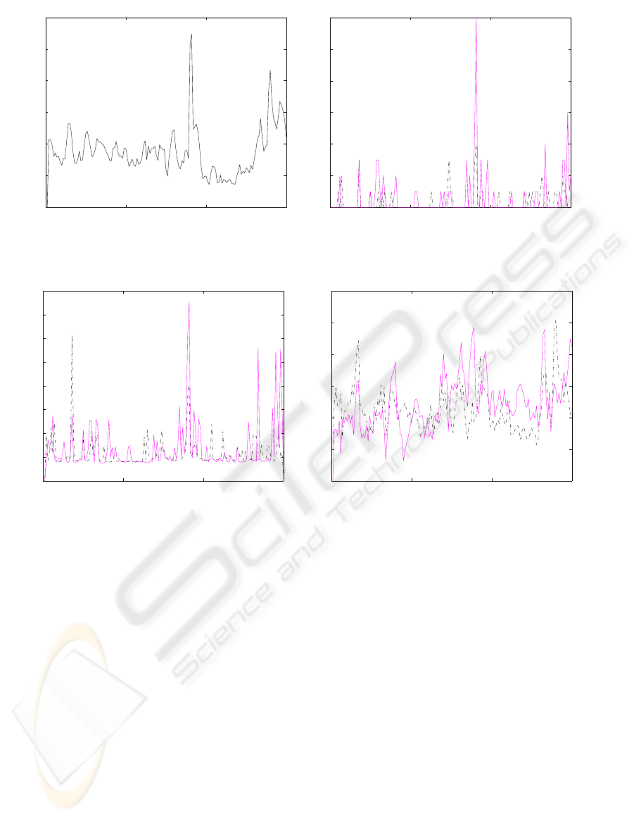
Figures 1 and 2 show some graphical informa-
tion about Foreman sequence and the application of
the binding of markers in two versions: the simple
one and the improved by the spatio-temporal gra-
dient - this one, using ∇
B
5
and W
B
4
as s.e.. Fig-
ure 1 (a) shows the amount of motion in Foreman se-
quence (computed by the symmetrical difference be-
tween consecutive frames) and Fig. 1 (b) shows the
number of user interferences for the two examples:
solid magenta plotting shows the number of interfer-
ences required in the simple binding of markers ap-
plication and the dot-dashed black plotting shows the
number of interferences for the spatio-temporal case.
Figure 2 (a) shows the plotting of the time needed
to segment each frame for the two example cases
(solid magenta plotting for the simple case, dot-
VISAPP 2010 - International Conference on Computer Vision Theory and Applications
168
0 50 100 150
0
0.01
0.02
0.03
0.04
0.05
0.06
(a)
0 50 100 150
0
2
4
6
8
10
12
(b)
Figure 1: Quantitative evaluation for Foreman sequence. (a) Motion information from Foreman sequence. (b) Number of
interferences for each frame.
0 50 100 150
0
5
10
15
20
25
30
35
40
(a)
0 50 100 150
0
0.5
1
1.5
2
2.5
3
(b)
Figure 2: Quantitative evaluation for Foreman sequence. (a) Time spent in each frame (secs.). (b) Segmentation error
(Percentile. Compared to the ground-truth).
dashed black plotting for the spatio-temporal one).
Note that the amount of efforts and time shown, re-
spectively in Fig. 1 (b) and Fig. 2 (a) are consistent
with the plotting with the image motion in Fig. 1 (a).
Finally, Fig. 2 (b) shows the plotting of the segmen-
tation error for each frame. In overall, the spatio-
temporal case had a lower error in most of the cases.
Figure 3 shows the segmentation of Foreman se-
quence using ∇
B
5
and W
B
4
. It is shown the segmen-
tation of the first 150 frames of the sequence.
4.2 Carphone Sequence
The segmentation of the man in Carphone sequence
is also a difficult task. Carphone is also a very used
sequence in the demonstration of image sequence
processing techniques. The goal in this experiment
was to segment the passenger from the remain of the
scene. The passenger moveshis body in several direc-
tions through the sequence, rotating slightly the body
and approaching the face to the camera in a given in-
stant. There are moments when the separation of the
left shoulder and the ear regions from the background
is difficult. More, the is also movement outside the
car window. The passenger is composed by several
objects: his head, which has difficult regions to seg-
ment and his hair, and the body, that is a easiest part
to segment. However, the region where the left shoul-
der meets the window has a low constrast and a strong
source of segmentation error.
Table 1 - Part Two shows the segmentation evalua-
tion of six experiments, the same applied to the Fore-
man sequence. Note that all mean segmentation er-
rors were close to 1%. The common binding of mark-
ers provided the best mean segmentation result, but
not too much better than the ones provided by the
spatio-temporal supported applications. Note, how-
ever, that the number of interferences decreased dras-
tically in the spatio-temporal gradient approaches:
simple binding of markers approach required 90 in-
terferences. The spatio-temporal approaches required
a third less effort to complete the task: they re-
WATERSHED FROM PROPAGATED MARKERS IMPROVED BY THE COMBINATION OF SPATIO-TEMPORAL
GRADIENT AND BINDING OF MARKERS HEURISTICS
169
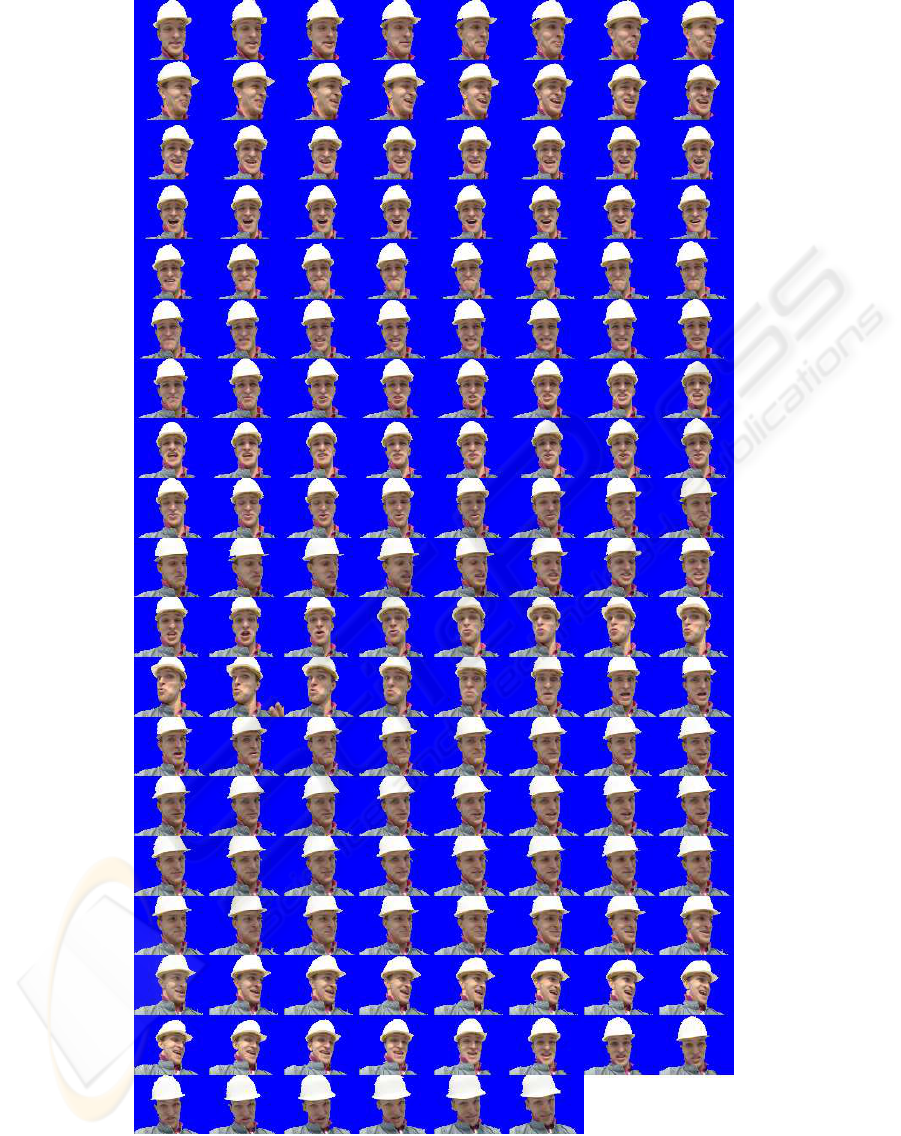
Figure 3: Segmentation of Foreman sequence (frames 1 to 150). Using ∇
B
5
and W
B
4
.
VISAPP 2010 - International Conference on Computer Vision Theory and Applications
170
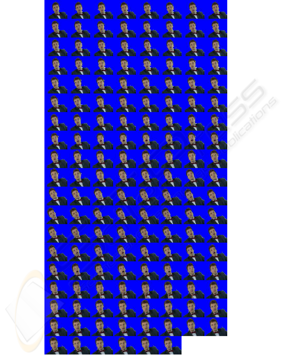
Figure 4: Segmentation of Carphone sequence (frames 1 to 150). Using ∇
B
17
and W
B
8
.
WATERSHED FROM PROPAGATED MARKERS IMPROVED BY THE COMBINATION OF SPATIO-TEMPORAL
GRADIENT AND BINDING OF MARKERS HEURISTICS
171

quired about 30 interferences, a very good improve-
ment compared to the simple binding of markers ap-
proach.
Figure 4 shows the segmentation of Carphone se-
quence using ∇
B
17
and W
B
8
. It is shown the segmen-
tation of the first 150 frames of the sequence.
5 CONCLUSIONS
This paper introduces an improvement to the wa-
tershed from propagated markers: the combination
of binding of markers heuristics with the spatio-
temporal gradient. The main idea consists in, for a
given frame, to apply the watershed from markers to
an image extracted from an 3-D gradient sequence,
computed by a morphological processing using a 3-
D s.e.. The applied markers were computed by the
binding of markers heuristics.
Experiments were done in order to assess the im-
pact of the addition of the spatio-temporal gradient
to the watershed from propagated markers framework
and this addition provided a increasing in the segmen-
tation performance. The decrease in the number of
interferences was significant and the quality of seg-
mentation was improved even with a lower number of
user interferences. Time segmentation decreased as
well.
Future works include the study of the spatio-
temporal gradient properties in order to improve the
segmentation results provided by the watershed from
propagated markers technique.
REFERENCES
B. Lucas and T. Kanade (1981). An interative image reg-
istration technique with an application to stereo sys-
tem. In Proceedings of DARPA Image Understanding
Workshop, pages 121–130.
Beucher, S. and Meyer, F. (1992). Mathematical Morphol-
ogy in Image Processing, chapter 12. The Morpholog-
ical Approach to Segmentation: The Watershed Trans-
formation, pages 433–481. Marcel Dekker.
B.K.P. Horn and B.G. Schunck (1981). Determining Optical
Flow. Artificial Intelligence, 17:185–204.
F. C. Flores, A. M. Polid´orio and R. A. Lotufo (2004).
Color Image Gradients for Morphological Segmenta-
tion: The Weighted Gradient Improved by Automatic
Imposition of Weights. In SIBGRAPI, pages 146–153,
Curitiba, Brazil.
F. C. Flores, A. M. Polid´orio and R. A. Lotufo (2006). The
Weighted Gradient: A Color Image Gradient Applied
to Morphological Segmentation. Journal of the Brazil-
ian Computer Society, 11(3):53–63.
F. C. Flores and R. A. Lotufo (2007). Watershed from
Propagated Markers Improved by a Marker Bind-
ing Heuristic. In G.J.F. Banon, J. B. and Braga-
Neto, U., editors, Mathematical Morphology and its
Applications to Image and Signal Processing, Proc.
ISMM’07, pages 313–323. MCT/INPE.
F. C. Flores and R. A. Lotufo (2008). Benchmark for Quan-
titative Evaluation of Assisted Object Segmentation
Methods to Image Sequences. In IEEE Proceedings
of SIBGRAPI’2008, pages 95–102, Campo Grande,
Brazil.
F. C. Flores and R. A. Lotufo (2009). Watershed from Prop-
agated Markers: An Interactive Method to Morpho-
logical Object Segmentation in Image Sequences. To
Appear on Image and Vision Computing.
F. Moscheni; Sushil Bhattacharjee and Murat Kunt (1998).
Spatiotemporal Segmentation Based on Region Merg-
ing. IEEE Transactions on Pattern Analysis and Ma-
chine Intelligence, 20(9):897–915.
Flores, F. C. and Lotufo, R. A. (2003). Object Segmenta-
tion in Image Sequences by Watershed from Markers:
A Generic Approach. In IEEE Proceedings of SIB-
GRAPI’2003, pages 347–352, Sao Carlos, Brazil.
Gonzalez, R. C. and Woods, R. E. (1992). Digital Image
Processing. Addison-Wesley Publishing Company.
J. L. Barron; D. J. Fleet and S. S. Beauchemin (1994). Per-
formance of Optical Flow Techniques. International
Journal of Computer Vision, 12(1):43–77.
P. Salembier et al (1997). Segmentation-Based Video Cod-
ing System Allowing the Manipulation of Objects.
IEEE Transactions on Circuits and Systems for Video
Technology, 7(1):60–74.
P. Smith; T. Drummond and R. Cipolla (2004). Layered
Motion Segmentation and Depth Ordering by Track-
ing Edges. IEEE Transactions on Pattern Analysis and
Machine Intelligence, 26(4):479–494.
S. S. Beauchemin and J. L. Barron (1995). The Com-
putation of Optical Flow. ACM Computing Surveys,
27(3):433–467.
Soille, P. and Vincent, L. (1990). Determining Watersheds
in Digital Pictures via Flooding Simulations. In Visual
Communications and Image Processing, pages 240–
250. SPIE. volume 1360.
VISAPP 2010 - International Conference on Computer Vision Theory and Applications
172
