
MULTISCALE VISUALIZATION OF RELATIONAL DATABASES
USING LAYERED ZOOM TREES AND PARTIAL DATA CUBES
Baoyuan Wang, Gang Chen, Jiajun Bu
College of Computer Science and Technology, Zhejiang University, Hangzhou, China
Yizhou Yu
University of Illinois at Urbana-Champaign, U.S.A.
Zhejiang University, Hangzhou, China
Keywords:
Database, Visualization, Data cubes, H-tree, GPGPUs.
Abstract:
The analysis and exploration necessary to gain deep understanding of large databases demand an intuitive and
informative human-computer interface. In this paper, we present a visualization system with a client-server
architecture for multiscale visualization of relational databases. The visual interface on the client supports
web-based remote access. We use zoom trees to represent the entire history of a zooming process that reveals
multiscale details. Every path in a zoom tree represents a zoom path and every node in the tree can have
an arbitrary number of subtrees to support arbitrary branching and backtracking. Zoom trees are seamlessly
integrated with a table-based overview using ”hyperlinks” embedded in the table. To support fast query pro-
cessing on the server, we further develop efficient GPU-based parallel algorithms for online data cubing and
CPU-based data clustering. Also, a user study was conducted to evaluate the effectiveness of our design.
1 INTRODUCTION
With increasing capabilities in data collection, large
databases are being produced at an unprecedented
rate. Examples include corporate data warehouses
archiving their operations such as sales and market-
ing, databases archiving historical climate changes,
historical census databases as well as large-scale gene
expression databases. A major undertaking with these
large-scale databases is to gain deeper understanding
of the data they contain: to identify structures and
patterns, discover anomalies, and reveal dependencies
and relationships.
The analysis and exploration necessary to achieve
these goals demand intuitive and informative human-
computer interfaces to these databases. There exist
challenges in developing such a powerful visual in-
terface. First, analysts working on databases often
need to see an overviewfirst, then progressivelyzoom
into details. How can we design an interface that
can seamlessly integrate overview and zoom capabil-
ities? Second, the path of exploration is unpredictable
and may rapidly change. Instead of predefined zoom
paths, the interface should be able to support dynami-
cally formed zoom paths. Furthermore, the history of
a zooming process should have a tree structure where
any node can have an arbitrary number of branches
for zooming into different local regions of the dataset.
How can we support arbitrary branching and back-
tracking in a zooming process and how can we ef-
fectively visualize the tree structure without wasting
screen space?
Data cubes are a common method for abstract-
ing and summarizing relational databases (Gray et al.,
1997). Cuboids in a data cube store pre-aggregated
results that enable efficient query processing and on-
line analytical processing (OLAP) (Chaudhuri and
Dayal, 1997; Mansmann and Scholl, 2007). Com-
putationally intensive aggregation is thus replaced
by fast lookup operations over the precomputed data
cube. By representing the database with a data cube,
one can quickly switch between different levels of de-
tail. However, for high-dimensional datasets, a fully
materialized data cube may be orders of magnitude
larger than the original dataset. It is only practical to
precompute a subset of the cuboids. Previous work
has demonstrated that online data cubing based on a
partial data cube can still significantly shorten query
response times. In the current context, a critical chal-
lenge with data abstraction is how to further reduce
101
Wang B., Chen G., Bu J. and Yu Y. (2010).
MULTISCALE VISUALIZATION OF RELATIONAL DATABASES USING LAYERED ZOOM TREES AND PARTIAL DATA CUBES.
In Proceedings of the International Conference on Imaging Theory and Applications and International Conference on Information Visualization Theory
and Applications, pages 101-111
DOI: 10.5220/0002829301010111
Copyright
c
SciTePress

query processing time to achieve interactive perfor-
mance using a partial data cube.
In this paper, we present solutions to the afore-
mentioned challenges and develop a complete visu-
alization system for multiscale visualization of rela-
tional databases. This paper has the following contri-
butions.
• We propose to use a tree structure called zoom
trees to represent the history of a zooming process
that revealsmultiscale details. Zoom trees support
arbitrary branching and backtracking.
• Zoom trees are seamlessly integrated with a table-
based overview using automatically generated
”hyperlinks” embedded in every chart of the ta-
ble. Once a user clicks any of these links, a new
zoom tree is initiated on a new layer.
• We further propose to use graphics processors
(GPUs) to perform real-time query processing
based on a partial data cube. We develop an ef-
ficient GPU-based parallel algorithm for online
cubing and a CPU-based algorithm for grid-based
data clustering to support such query processing.
• We integrate all components together into a com-
plete client-server system. The client is Flash
based and supports web-based remote access.
Queries and processing results are communicated
between the client and server via a network con-
nection. Queries are automatically generated ac-
cording to user interactions.
2 RELATED WORK
2.1 Multi-Dimensional Dataset
Visualization
Over the decades, much work (Antis et al., 1996;
Weijia Xu, 2008) has been done on visualizing
relational database to uncover hidden casual rela-
tions. Lots of visualization techniques for multi-
dimensional datasets have been designed including
parallel coordinates, scatter plot matrices, and dense-
pixel display.
Recently, more and more databases are augmented
with data cubes which provide meaningful levels of
abstraction. To integrate humans into the exploration
process and uncover the hidden patterns more intu-
itively and easily, lots of data cube visualization tech-
niques have been developed. A pioneering database
visualization system called Polaris (Stolte et al., 2002)
visually extends the Pivot table (Inc, 2007) by using
various graphical marks instead of text. It provides
multiscale cube visualization in the form of zoom
graphs and four design patterns (Stolte et al., 2003).
However, the drawbacks of polaris include poor scal-
ability over large datasets and only predefined zoom
graphs are supported. The meaning of scalability is
twofold. It refers to both query response time and
screen space clutter over large datasets. The visu-
alization system in this paper overcomes these lim-
itations. (Maniatis et al., 2003) proposed a method
to map the cube presentation model (CPM) to Ta-
ble Lens (Rao and Card, 1994), which is a well-
known distortion technique. Based on hierarchical
dimensional visualization (HDDV (Kesaraporn et al.,
2004)), (Techapichetvanich and Datta, 2005) pro-
posed an interactive cube visualization framework
which uses horizontal stack bars to represent dimen-
sions, and roll-up and drill-down operations are im-
plemented through directly manipulating these bars.
(Pro, ) was the first to introduce a hierarchical drill-
down visualization called decomposition trees, based
on which (Mansmann and Scholl, 2007) introduced
enhanced decomposition trees. Our proposed hier-
archical zooming technique is partially inspired by
(Rep, ), which provides a web-based reporting solu-
tion. The client offers different types of chart trees,
and drill-down operations are implemented by ex-
panding specified bars along potentially different di-
mensions. Semantic zooming interfaces were devel-
oped in Pad++ (Bederson and Hollan, 1994), DataS-
plash (Allison et al., 2001) and XmdvToll (Runden-
steiner et al., 2002).
One challenging problem facing visualization sys-
tems is their scalability with large datasets because an
overcrowded visual presentation has a negative im-
pact on the analysis process. To reduce clutter and
make visualizations more informative to end-users, a
variety of techniques and algorithms have been de-
signed. (Fua et al., 1999; Kreuseler and Schumann,
1999) proposed a multiresolutional view of data via
a hierarchical clustering method for parallel coordi-
nates. (Peng et al., 2004) proposed to use dimension
reordering for a variety of visualization techniques in-
cluding star glyph and scatter plots. However, to the
best of our knowledge, no clustering techniques have
been proposed to support charting large datasets, es-
pecially for plot charts. A taxonomy of clutter reduc-
tion for visualization can be found in (Ellis and Dix,
2007).
2.2 Data Cubes
Data cubes categorize database fields into two classes:
dimensions and measures, corresponding to the in-
dependent and dependent variables, respectively. A
IVAPP 2010 - International Conference on Information Visualization Theory and Applications
102
data cube consists of a lattice of cuboids, each of
which corresponds to a unique data abstraction of the
raw data. A data abstraction is defined by a specific
projection of the dimensions. A cuboid is abstractly
structured as an n-dimensional cube. Each axis cor-
responds to a dimension in the cuboid and consists of
every possible value for that dimension. Each ”cell”
in the cuboid corresponds to a unique combination of
values for the dimensions. Each ”cell” also contains
one value per measure of the cuboid. H-tree based
cubing was initially proposed by (Han et al., 2001) for
iceberg cubes and later extended to support stream-
ing data (Han et al., 2005). In this paper, we develop
a technique for interactively exploring the aggregates
by using an H-tree as a partially materialized cube.
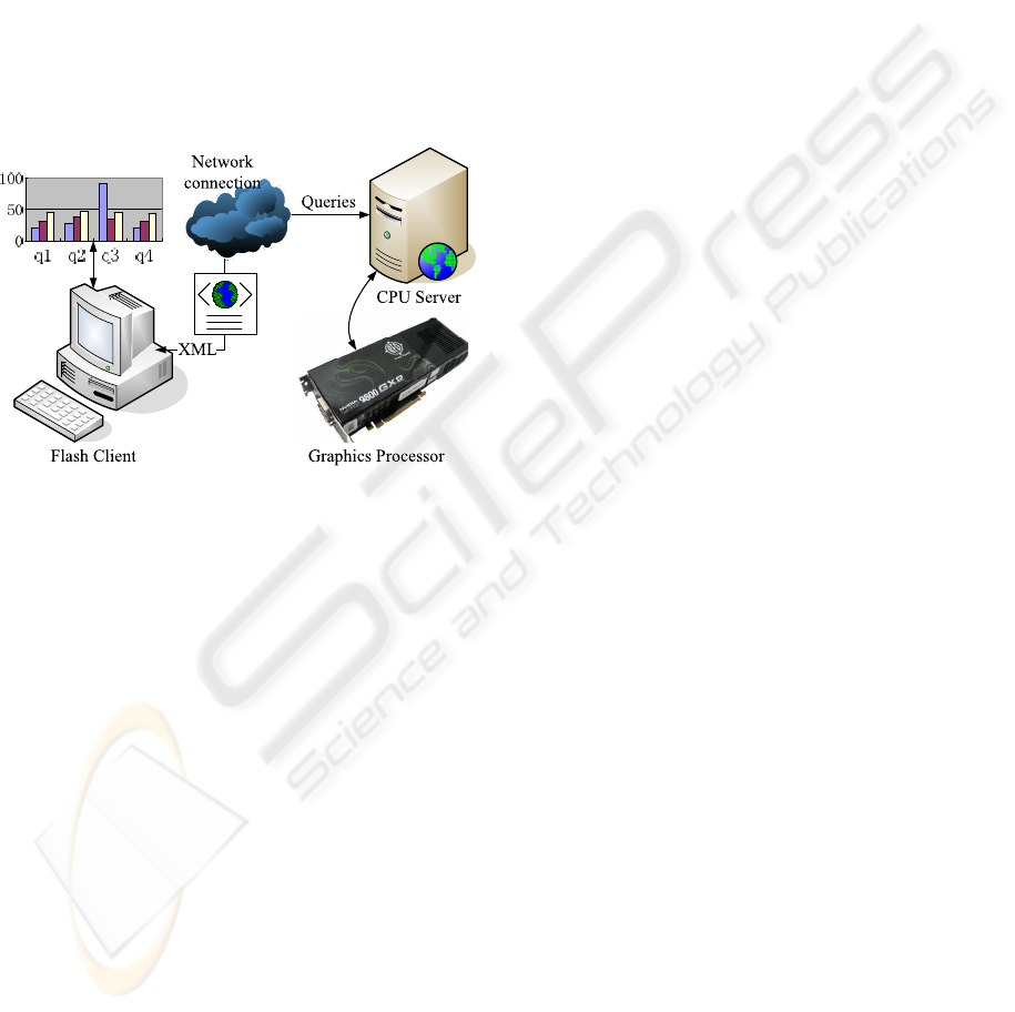
Figure 1: System Architecture.
3 SYSTEM ARCHITECTURE
We adopt the classic client-server architecture for our
visualization system (Figure 1). We chose to develop
the visual interface in Flash on the client side. Flash
exhibits multiple advantages in this task. First, it is
cross-platform and can be easily embedded into most
of the web browsers. Furthermore, flash code written
in ActionScript is interpreted and executed at run time
by the Flash Player which is commonly preinstalled
on personal computers. This makes our visualiza-
tion system web-based and readily availableto remote
users. Second, ActionScript, the scripting language
for Flash, facilitates user interface development and
has a charting component that supports the drawing
of basic charts, including bar charts, pie charts, and
plot charts, which are among the elementary building
blocks of our visual interface.
Our visual interface supports a wide variety of
user interactions to help the user visually analyze the
database under consideration. Most of these interac-
tions are transformed into a number of queries ac-
cording to a predefined formalism. Then all these
queries are sent to the server via a network connec-
tion. The server has both a CPU component and a
GPU component. The CPU component is mainly re-
sponsible for data clustering and communication with
the client while the GPU component, which serves as
a coprocessor, performs most of the computationally
intensive tasks, including query processing and data
bounding box evaluation. The processing results are
formatted into an XML file on the CPU and sent back
to the client.
4 VISUAL INTERFACE
In this section, we introduce our proposed visual ab-
straction. We would like to achieve the following
overall design goals.
1. Dense display of various types of charts for effi-
cient utilization of the screen space
2. Interactive subcube selection for setting focus of
the analysis
3. A powerful and flexible zoom interface for detail
investigation
We address these design goals by incorporating three
main user interface components, schema-based nav-
igation for subcube selection, a table-based layout
for an overview of the selected subcube, and layered
zoom trees for the exploration of details. We elabo-
rate these components in the following subsections.
4.1 Schema based Subcube Selection
Instead of analyzing the entire data cube at once, users
usually would like to focus on a subset of the dimen-
sions every time. A subcube is defined by a subset
of the dimensions. Each of the remaining dimensions
is fixed to a specific value. In a data cube, a sub-
cube can be specified with slice/dice operations. In
our system, slice/dice operations are implemented us-
ing the schema list shown in a control panel (Fig. 2).
The schema is visualized as a hierarchical tree struc-
ture with each dimension represented as a node in the
tree. If a user left-clicks a node, all the possible val-
ues of the dimension are presented in a pop-up list.
The user can choose whatever value by clicking the
corresponding check-box to the left of the value. A
slice operation performs a selection on one of the di-
mensions while a dice operation defines a subcube by
performing two or more slice operations. Users can
perform either operations on the schema. (Mansmann
and Scholl, 2007) proposed a similar schema naviga-
tion. However, there is a major difference between
MULTISCALE VISUALIZATION OF RELATIONAL DATABASES USING LAYERED ZOOM TREES AND
PARTIAL DATA CUBES
103

(a) (b) (c)
Figure 2: Schema based subcube selection. (a) shows the
initial stage. If the user would like to view a slice of the
data for the state, ”Florida”, he descends into the ”Location”
hierarchy, clicks the ”States” node, and selects ”Florida” in
the pop-up list shown in (c).
them. For a dimension with an overly large cardinal-
ity, our system automatically builds a hierarchical list
for distinct values in the dimension so that an item at
an intermediate level represents a range of values. It
would be impossible to show all values in the dimen-
sion on the screen without such a hierarchical list.
4.2 Table based Overview
Once a target subcube has been selected, the user can
generate an overview of the subcube by configuring
the axes of a 2D table-based visualization component
which was inspired by Polaris (Stolte et al., 2002)
and Pivot Table (Inc, 2007). The table based visu-
alization is able to reveal high-level trends and corre-
lations in the chosen subcube. More detailed infor-
mation can be progressively fetched through zoom-
ing or drill-down operations. Unlike Polaris, at most
two nested database dimensions (measures) can be
mapped along the horizontal or vertical direction of
the table to achieve simplicity and clarity. Four pull-
down lists on the interface allow the user to configure
the table by choosing the dimensions and measures
assigned to the two outer axes and two inner axes and
the visual presentation is automatically determined by
the configuration of these axes (Fig. 3).
As usual, our table-based overview supports vari-
ous interactive operations on data cubes. Such oper-
ations include pivoting, roll-up, drill-down, filtering
and sorting. To facilitate side-by-side comparisons,
the user can also reorder rows and columns in the ta-
ble by dragging desired ones together.
4.3 Zoom Trees for Detail Visualization
Zooming is a frequently used operation in visualiz-
ing multi-dimensional relational databases and data
cubes. In this section we propose to use zoom trees
on separate layers for facilitating the presentation of
zooming results along with the zooming history.
4.3.1 Layered Zoom Trees
Given an overview of a selected subcube in our table-
based visualization component, visual analysts typi-
cally need to dig deeper into the subcube to gain more
insights or discover correlations and anomalies. Since
the table-based overview can only accommodate up to
four dimensions/measures, the remaining dimensions
are aggregated together. To discover more details,
zooming needs to disaggregate such dimensions or
expand an existing dimension to expose more detailed
levels. A zooming process in our system is purely
event driven, and it always begins with a chart in the
table-based overview. The events embedded into the
chart (in the table) serve as ”hyperlinks”. For exam-
ple, a user can initiate a zooming process by clicking
any bar in a bar chart or select a region of interest in
a plot chart in the table (Fig. 4). Any event triggered
by such user interactions pops up a new active layer.
The chart clicked by the user becomes the root of a
new zoom tree initiated on this layer, and the disag-
gregated information corresponding to the chosen bar
or region is presented in a new chart, which becomes
a child of the root. The user can continue to zoom into
any existing node in this tree, and a new child of the
existing node is spawn holding the zooming results.
To reduce screen space clutter, at any time, only
one path from the root to a leaf in the tree is visu-
alized, and all other nodes in the tree are hidden. A
path in a zoom tree is presented in a predefined layout
within the layer, where the nodes are arranged from
left to right horizontally and from top to bottom verti-
cally. Each node in the tree is a chart, and represents
a disaggregation of a dimension or an intermediate
level of a hierarchically clustered dataset. A user can
dynamically change the type of chart shown within a
node. The user can also minimize (deactivate) and re-
activate a layer. There can be only one active layer at
any time.
There are three operations supported for zoom
trees.
1. Add nodes. Double-click a bar or a pie or select
a region in a plot chart, a list of dimensions will
pop up. Once the user has chosen one of the di-
mensions, a new chart will be generated as a new
child node.
2. Delete nodes. Nodes can be deleted by directly
clicking the ”Delete” button on each chart. If a
node is deleted, all its descendants are pruned at
the same time.
3. Show/Hide nodes. Since our system only shows
one path from the root to a leaf in the tree, the
user can choose a desired branch by clicking the
radio button representing the root of the subtree.
IVAPP 2010 - International Conference on Information Visualization Theory and Applications
104

Figure 3: Overview of the visual interface. The schema list is in the left panel. There are four pull-down lists at the top of
the right panel for table configuration. Minimized zoom trees are listed at the bottom of the window. The above screenshot
visualizes census information of Illinois, including statistics on education, occupation, income, industry and so on.
All sibling nodes of the chosen branch and their
decedents become all hidden.
Compared with decomposition trees in (Mans-
mann and Scholl, 2007) and semantic zooming in
the Pad++ system (Bederson and Hollan, 1994), our
zoom trees have two unique characteristics. First, a
zoom tree has a generic tree structure recording the
entire history of a zooming process performed on a
chart in the overview. Unlike previouswork, a node in
a zoom tree can have an arbitrary number of children.
But at any time there is only one child visualized to
efficiently utilize screen space. Second, pivoting is
supported during a zooming process. It provides ad-
ditional dynamic views of the data and, therefore, hid-
den patterns could be discovered more easily. There
are two types of zooming according to the data type
it operates on. One is for data with aggregated di-
mensions and the other is for data clusters which are
computed from either raw or aggregated data points
to reduce screen space clutter.
4.3.2 Zooming Aggregated Data
This type of zooming applies to bar charts and other
types of charts essentially equivalent to bar charts,
such as pie charts and line charts. During a zoom-
ing step, the user chooses a bar and disaggregates it
along a dimension that is different from the dimension
mapped to one of the axes of the chart (Fig. 4(a)&(c)-
(e)). Note that different bars in the same chart can
be disaggregated along different dimensions. Such
a zooming step essentially performs local drill-down
over a subset of aggregated data. The flexibility of
such zooming steps facilitates detailed data explo-
ration.
4.3.3 Zooming Data Clusters in Plot Charts
There can be a huge number of data points in a plot
chart while the screen area allocated for the chart is
often quite limited. Overly crowded points in a plot
chart can prevent users from identifying the underly-
ing correlations and patterns. To reduce this type of
screen space clutter, we perform clustering on the data
points using screen space distance, and only visual-
ize the cluster centers in the plot chart. Every cluster
center is visualized as a small circle whole radius in-
dicates the number of data points in the underlying
cluster. The clustering algorithm is executed on the
CPU which takes the screen location of the raw data
points and the number of desired clusters as input (see
Section 6.2). Zooming such data clusters can be initi-
MULTISCALE VISUALIZATION OF RELATIONAL DATABASES USING LAYERED ZOOM TREES AND
PARTIAL DATA CUBES
105

(a) (b)
(c) (d)
(e) (f)
Figure 4: (a)&(c)-(e) show a series of screenshots for a multiscale visualization of a coffee chain database, which has been
abstracted into an eight dimensional partial data cube. The table in (a) has the sixth type of configuration stated in Section
4.2. When a user would like to disaggregate ”Profit” in ”February”, he should left-click the corresponding ”pie” of the pie
chart in the top-left pane. He will be presented a list of aggregated dimensions. The user selects ”Market” as the dimension to
be disaggregated, and a new zoom tree will be initiated. (c)-(e) show three different views of this zoom tree. The view in (d)
is obtained by pivoting the second node from ”MarketType” to ”Product”. And (e) is obtained by clicking the second branch
from the root. This operation automatically hides the first subtree of the root. Note that there is a caption in the header of
each node to indicate its scope. (b)&(f) show two screenshots with plot charts visualizing historical climate records including
”Temperature”, ”Precipitation”, and ”Solar Radiation” in US during the last century. Such visualizations enable analysts to
discover potential relationships among these measurements. The view in (f) is obtained by zooming into a region in a pane of
the table in (b). Note that the views in (c)-(f) are displayed on pop-up layers above the original table.
ated by drawing a rectangular region of interest (Fig.
4(b)&(f)). Cluster centers falling into the region are
automatically selected. A new chart is created as a
child of the current node in the zoom tree displaying a
zoomed view of the region. This zoomed view is gen-
erated on the fly by calling the clustering algorithm on
the server again over those raw data points falling into
the selected region. Because the selected region is
zoomed to cover the area of an entire chart, the num-
ber of resulting cluster centers becomes larger than
that in the selected region of the original chart. Such
a zooming step can be recursively performed until the
number of raw data points within the region is less
than a threshold. Note that zooming clustered data
does not involve any aggregated dimensions.
4.3.4 Pivoting During Zooming
It would be desired to gain more insight during data
analysis by generating additional views of a node in
a zoom tree. Users can achieve this goal with the
help of pivoting. Unlike pivoting discussed in Sec-
tion 4.2 where the axis configuration of the entire ta-
ble is changed, pivoting here is only applied locally to
IVAPP 2010 - International Conference on Information Visualization Theory and Applications
106

a chart in a particular tree node and can be performed
on any node in the zoom tree. For this purpose, users
can directly click the pull-down list along the dimen-
sion axis of the chart and choose the desired dimen-
sion for the new view. We restrict the target dimen-
sion for pivoting to be selected from the remaining
dimensions which have not been used so far.
5 QUERY FORMATION
In this section, we briefly discuss how to transform
user interactions into queries and how these queries
are expressed according to a predefined formalism.
5.1 Query Formalism
Since we adopt the H-Tree (Han et al., 2001) as
the implementation of our partial cube, typical cube
query languages such as MDX can not be used to de-
scribe a query. Therefore we develop a simple H-
tree based partial cube query formalism. Generally,
there are two kinds of queries for data cubes:(1) point
query and (2) subcube query. A point query only in-
cludes a few instantiated dimensions but without any
inquired dimensions. On the other hand, a subcube
query is required to include at least one inquired di-
mension. We use ”?” to represent an inquired dimen-
sion, ”*” to represent a ”Not care” dimension, and a
string of values demarcated by slash(”/”) to represent
an instantiated dimension. Assume the partial cube is
constructed from a relational database with M dimen-
sions and K measures. There exists a predefined order
of the dimensions, D
1
,D
2
,...,D
M
, typically specified
by OLAP experts. In such a context, the two kinds of
queries can be expressed in a formalism used by the
following two examples:
< ∗,∗,d
31
/d
33
,∗,...,∗; m
j1
,...,m
ji
,...,m
jK
>, (1)
< ∗,?,d
51
/d
57
,?,...,∗; m
j1
,...,m
ji
,...,m
jK
>, (2)
where m
ji
(1 ≤ i ≤ K) represents the label of a mea-
sure, m
ji
= 1 if it is inquired otherwise it is set to 0;
d
31
and d
33
are two specified values for the instan-
tiated third dimension. There are two parts in each
query. The first part is reserved for the dimensions
demarcated by commas(”,”) and the second part is for
the labels of the measures also demarcated by com-
mas. Note that there could be more than one val-
ues specified for each instantiated dimension. (1) de-
scribes a point query, which returns one aggregated
value for each inquired measure. (2) describes a sub-
cube query with the second and fourth dimensions as
inquired dimensions.
5.2 Query Generation
Queries similar to (1) and (2) are generated by tracing
user interactions and filling slots corresponding to di-
mensions relevant to the interactions. Note that, there
can be only three types of values for each slot: ”*”,
”?” or a string of instantiated values.
Slice/Dice Selection. As discussed in Section 4.1,
slice and dice only specify instantiated dimensions.
Thus, values of the instantiated dimensions will be di-
rectly filled into the corresponding slots of the query.
For example, if we selected ”2007” and ”2008” as the
values for the dimension ”Year”, the ”Year” slot will
be filled with ”2007/2008” in all subsequent queries.
Query Generation for Table-based Overview. As
stated in Section 4.2, four of the six types of com-
monly used axis configuration generate tables of
charts, and the other two generate a single large bar
chart or plot chart. In the first type of configuration
mentioned in Section 4.2, there is only one dimension
specified, therefore, only one subcube query is gener-
ated taking the dimension assigned to the outer ver-
tical axis as the inquired dimension and all the mea-
sures as the inquired measures. The second type of
configuration is a special case of the first one since it
only inquires one measure. A 2D table can be gen-
erated by assigning two dimensions to the two outer
axes. Once specified, the whole table is divided into
a 2D grid of panes each of which maps to a specific
pair of values of the dimensions assigned to the outer
axes. A subcube query is generated for each pane.
The actual query type depends on whether there is a
dimension assigned to the inner axes. For instance,
in the fourth type of configuration in Section 4.2, one
subcube query is generated for each pane taking the
inner horizontal dimension as the inquired dimension.
In the fifth type of configuration, one subcube query
is generated for each pane taking the two inner mea-
sures as inquired measures and all uninstantiated di-
mensions as inquired dimensions.
Query Generation for Zooming and Pivoting.
Zooming aggregated data needs to unfold new dimen-
sions. Every aggregated datum is decomposed into
multiple ones each of which corresponds to a dis-
tinct value of the dimension chosen for disaggrega-
tion. Therefore, only one subcube query is generated
for each such operation taking the chosen dimension
as the inquired dimension. Similarly, a pivoting oper-
ation is also transformed to one subcube query. How-
ever, zooming clustered data is different in that no ad-
ditional dimensions are required. When the user se-
lects one region of interest to zoom in, the system au-
tomatically computes the bounding box of the region.
MULTISCALE VISUALIZATION OF RELATIONAL DATABASES USING LAYERED ZOOM TREES AND
PARTIAL DATA CUBES
107

This bounding box is appended to the query corre-
sponding to the pane. The query will be processed
as usual except that query results will be filtered us-
ing the bounding box and the filtered results will be
re-clustered.
Subcube Query Translation. In our system, a sub-
cube query is first translated into multiple point
queries before being further processed. The idea is
to replace all inquired dimensions in the query with
all possible combinations of their values. More pre-
cisely, if there are n inquired dimensions in the query
with cardinalityC
1
,...,C
n
respectively, it will be trans-
lated into
∏
n
i=0
C
i
point queries each of which maps to
a unique combination of values of these inquired di-
mensions. To minimize data transmission overhead,
the translation is performed by the CPU component
of the server.
6 SERVER-SIDE ALGORITHMS
In this section, we present algorithms developed for
the server.
We adopt an H-tree to represent the partially ma-
terialized data cube on the server. H-tree is a hyper-
linked tree structure originally presented in (Han
et al., 2001), and was later deployed in (Han et al.,
2005) as the primary data structure for stream cubes.
However there are two major differences in our GPU-
Figure 5: GPU H-tree Structure.
based H-tree structure (Fig. 5) compared with the
original version. First, since CUDA does not sup-
port pointers, linked lists are replaced with arrays and
pointers are replaced with array indices. Second, the
array allocated for a side-link list is further divided
into contiguous segments each of which contains in-
dices of nodes which share the same attribute value.
We revised the structure of side links to achieve better
load balance and query performance.
Recently, GPUs attract more and more attentions
beyond the graphics community. Take the advantage
of the GPU H-tree structure, we develop a parallel
approach of online cubing algorithm to facilitate fast
query processing. We adopt NVidia CUDA (CUDA,
2008) as our programming environment. This is the
first attempt to develop parallel cubing algorithms on
GPUs to the best of our knowledge.
6.1 Online Cubing
In this section, we only present the GPU-based par-
allel algorithm for point queries because a subcube
query can be easily translated into multiple point
queries. To achieve optimal performance, we propose
an approach exposing two levels of parallelism. Un-
like a sequential algorithm which processes queries
one by one, our algorithm can process thousands of
queries simultaneously in parallel. To further exploit
the massive parallelism of modern GPUs, we make
each query processed in parallel. We achieve this goal
by first assigning one thread block to each query and
then making each thread in the block responsible for
an evenly divided portion of leaves or intermediate
nodes of the H-tree. Since each query is processed
by one thread block, we present the per-block query
processing algorithm as follows.
Algorithm: POINT QUERY
Input: HT, an H-tree;
pq, a point query including a set of instanti-
ated dimensions and a set of inquired measures;
Output: An aggregated value for each inquired
measure.
variables: i ← 0
begin
1. Follow the predefined order of dimensions, locate
the last instantiated dimension, hd, in pq; load pq
and the header table for dimension hd into the shared
memory of the current thread block.
2. Search the header table for the i−th specified value
of hd in pq to retrieve the number of its repetitions,
rNum, and the index of its first occurrence, start, in
the corresponding side-link list.
3. For each element e in the interval [start,start +
rNum] of this side-link list in parallel, locate the node
in the H-tree corresponding to e and use its parent in-
dex to move up the tree while checking all the instan-
tiated dimensions on the way. If one specified value of
every instantiated dimension can be found along the
path, fetch the values of the inquired measures stored
in the node corresponding to e and insert the value of
each inquired measure into a distinct temporary array.
IVAPP 2010 - International Conference on Information Visualization Theory and Applications
108

i+ = 1, go to step 2.
4. Perform parallel reduction on the temporary ar-
ray for each inquired measure to obtain the final ag-
gregated value for each inquired measure.
end
In a real scenario, we initiate thousands of thread
blocks and each block takes care of one query. Note
that, in the first step we assume that the entire header
table for hd and the query itself can be completely
loaded into the shared memory associated with the
block responsible for the query. Much care should be
taken to make sure it would not exceed the maximal
limit, which is 16KB per stream processor on G80.
If the cardinality of hd is relatively large, step 2 can
be parallelized as well. In step 3, we evenly divide
the rNum elements in the side-link list into chunks,
and the size of each chunk is rNum/S, where S is the
number of threads in a block. We allocate a tempo-
rary array for each inquired measure. Each element
in this array represents a partially aggregated value
computed from a particular chunk by the correspond-
ing thread. Since there could be more than one speci-
fied values for the last instantiated dimension, we loop
over all these values and accumulate all partially ag-
gregated values to the temporary arrays. Finally, we
apply the parallel reduction primitive (Harris, 2008)
to each temporary array to compute the final aggre-
gated value for each inquired measure.
The average time complexity of online cubing is
O(NM/(CP)) per point query, where P is the number
of processors allocated to process the query, N is the
number of tuples in the H-tree, M is the number of
dimensions, and C is the cardinality of the last instan-
tiated dimension in the query. The memory cost of
online cubing is O(S) per point query, where S is the
number of threads responsible for the query.
6.2 Online Clustering for Plot Charts
Implementing the zooming mechanism described in
Section 4.3.3 for plot charts requires performing clus-
tering in real time on the server. Classical clustering
methods such as K-means could be used for this pur-
pose. However, the main drawback of the k-means
algorithm in this scenario is that it requires multiple
iterations to cluster the data into a desired number of
clusters, which makes it hard to achieve real-time re-
sponse for large datasets even if we use its parallel
version (Shalom et al., 2008). Here we present a sim-
ple grid-based algorithm to cluster hundreds of thou-
sands of points into a desired number of clusters. In
doing do, we can not only reduce the overhead for
transferring a large amount of data but also can reduce
screen space clutter. To deliver optimal performance,
our clustering algorithm has been implemented on the
CPU of the server and is summarized in the following
steps.
1. Compute the bounding box of all input points.
2. Divide the bounding box into a 2D grid of N
bin
×
N
bin
small boxes with equal size. Each small box
serves as a bucket.
3. Accumulate each point into an appropriate bucket
according to its screen space coordinates.
4. for every bucket in the grid, set the cluster center
of the bucket at the average location of the points
falling into the bucket.
This algorithm has a linear time and space com-
plexity. A reasonable value for N
bin
is 10. Users can
tune this parameter to achieve a visually pleasing pre-
sentation.
6.3 Performance
The described algorithms have been implemented and
tested on an Intel Core 2 Duo quad-core 2.4GHz pro-
cessor with an NVidia GeForce 8800 GTX GPU. To
cluster 1 millon randomly generated data points into
10x10 clusters, our grid-based clustering algorithm
only takes 22.96ms on a single core. The average
performance of the on-line cubing algorithm is pre-
sented in Fig. 6(a)&(b), where randomly generated
point queries are processed using an H-tree with 400k
and 800k tuples, respectively. Our GPU-based algo-
rithm can typically achieve a speedup much larger
than 10, and process 10,000 to 50,000 point queries
per second. The results also show that this algorithm
has more advantages when the number of dimensions
and the cardinality of each dimension are relatively
small. This is mainly because more dimensions and a
larger cardinality of the dimensions give rise to larger
H-trees which require more memory accesses. GPU
memory access latency is about 400-600 cycles which
is longer than CPU DRAM access latency.
6 9 12 15 18
0
0.1
0.2
0.3
0.4
0.5
0.6
0.7
0.8
0.9
# of dimension
Per Query Elapsed time(ms)
On Line Cubing Query for C160T800K
CPU
GPU
Speedup
0
5
10
15
20
25
30
35
40
45
50
Speedup
20 40 80 160 320
0
1
2
3
4
5
6
7
Cardinality
Per Query Elapsed time(ms)
On Line Cubing for D15T400K
CPU
GPU
Speedup
0
2
4
6
8
10
12
14
16
18
20
Speedup
(a) (b)
Figure 6: GPU speedup and average time vs. # of dimen-
sions and the cardinality of each dimension for online cub-
ing.
MULTISCALE VISUALIZATION OF RELATIONAL DATABASES USING LAYERED ZOOM TREES AND
PARTIAL DATA CUBES
109

7 USABILITY EVALUATION
To evaluate the usability of our system, we explored
several real datasets, including the American histor-
ical climate changes data of the last century and the
American census data in 2000 as well as the Coffee
Chain data(shown in the video). Since polaris can
be treated as the state-of-art for database visualiza-
tion, a user study was then conducted by comparing
the visualizations of these datasets using both zoom
tree and Tableau(Polaris). There were 8 total partici-
pants: 2 female,6 male. Their ages ranged from 19 -
28. They were from four different research labs, in-
cluding database(2), data mining(2), graphics(2) and
HCI(2).
7.1 Methods and Procedure
Before the testing, about one hour training and dis-
cussion were conducted in order to make them all
familiar with the meanings of datasets, the concepts
of cube as well as the interfaces of the two systems.
Participants were asked to perform two tasks with
both systems and rate(1-5) their satisfactions by fill-
ing out questions. Note that, both tasks were in-
volved drilling down, rolling up and pivoting oper-
ations. An example step of one task is like: Se-
lect the sub-cube: ”Year=2007, Location=NewYork,
Product=Green Tea, then explore and find the abnor-
mal relationships between the remaining dimensions
and the measure ’Profit’ and then record them down.”.
An example of the questions is like: Rating the satis-
faction about the pivoting support along a zoom path.
7.2 Results and Observations
We measured the tasks times costed by each par-
ticipant. The average and variance time for task
one and two used by zoom tree are (average =
36s,variance = 15s) and (average = 95s,variance =
24s) respectively. While the corresponding results
used by polaris for the two tasks are (average =
45s,variance = 12s) and (average = 87s,variance =
26s) respectively. We also report the user satisfac-
tion ratings for the two different systems through ta-
ble 1. From the qualitative results including both pos-
itive and negative feedbacks, we found our system is
competitive with Polaris. Intuitive, easy to invoke and
manipulate, less clutter for high dimensional data all
make the layered zoom tree powerful. An interest-
ing observation is that most of the participants agree
table is good for overview visualization, but details
should be better visualized gradually in an isolated
layer to achieve clarity if focus and context is well
Table 1: User Satisfaction Ratings(0:Worst, 5:Best).
Question Zoom Tree Polaris
Subcube Selection 3.7 3.9
Pivoting 4.6 3.5
Aesthetic Appeal 3.4 3.7
Clutter Reduction 3.9 3.3
System Response Time 4.3 4.1
Historical Vis Support 3.8 3.7
processed. According to our experience, it’s really
hard to visualize datasets with 15 dimensions above
in a fixed table using dimension embedding as in po-
laris, the higher the dimension the more clutter the
visualization. This is one of the main drawbacks of
polaris that layered zoom tree avoided. The results
also show that zoom tree gives quicker response time
for the same dataset, that’s mainly due to the leverage
of GPU parallelism through our H-tree online cubing
algorithm. Moreover, zoom tree only stores a partial
cube, compared with Polaris, it will save much more
spatial space. Flexibly changing the view is crucial
for users to facilitate the dynamic exploration, since
pivoting is not supported along the zoom path in po-
laris, layered zoom tree is absolutely the winner with
regard to this.
However, zoom tree also has some disadvantages,
for example participants think that although schema
based subcube selection is powerful, they prefer di-
rectly dragging and dropping dimensions to the table
shelves as in polaris. We also received some valu-
able suggestions for further improvement. For exam-
ple, one suggested to annotate the history button into
a meaningful thumbnail which reveals the structure of
the underlying subtree.
8 CONCLUSIONS
We have presented a visualization system with a
client-server architecture for multiscale visualization
of relational databases. Our system supports all types
of data cube operations using a combination of a
schema list, tables and zoom trees. To support fast
query processing on the server, we have also de-
veloped efficient algorithms for online data cubing
and data clustering. The user study shows that our
proposed layered zoom tree and the overall system
framework are effective for visualizing databases.
Limitation. Our current system does not support
spatial dimensions such as maps. A spatial dimension
is likely to partition the screen space into irregularly
shaped regions instead of regularly shaped panes. In
future, we would be interested in investigating meth-
ods for placing charts inside such regions as well as
IVAPP 2010 - International Conference on Information Visualization Theory and Applications
110

zoom interfaces for spatial dimensions.
ACKNOWLEDGEMENTS
We would like to thank Shaowen Wang for the his-
torical climate dataset, Jiawei Han and Pat Han-
rahan for helpful discussions and suggestions, and
the anonymous reviewers for valuable comments.
This work was partially supported by NSF (IIS
09-14631), National Natural Science Foundation of
China (60728204/F020404).
REFERENCES
Proclarity analytics 6 2006. from: http://www.proclarity.
com/products/proclarity analytics 6.asp.
Report portal 2006:zero-footprint olap web client solution
xmla consluting. from:. http://www.reportportal.com.
Allison, W., Chris, O., Alexander, A., Michael, C., Vuk,
E., Mark, L., Mybrid, S., and Michael, S. (2001).
Datasplash: A direct manipulation environment for
programming semantic zoom visualizations of tabu-
lar data. Journal of Visual Languages & Computing,
12:551–571.
Antis, J., Eick, S., and Pyrce, J. (1996). Visualizing
the structure of large relational databases. Software,
IEEE, 13(1):72–79.
Bederson, B. B. and Hollan, J. D. (1994). Pad++: a zoom-
ing graphical interface for exploring alternate inter-
face physics. In UIST ’94: ACM symposium on user
interface software and technology.
Chaudhuri, S. and Dayal, U. (1997). An overview of
data warehousing and OLAP technology. SIGMOD
Record, 26:65–74.
CUDA (2008). Nvidia cuda (compute unified de-
vice architecture) programming guide 2.0.
http://developer.nvidia.com/object/cuda.html.
Ellis, G. and Dix, A. (2007). A taxonomy of clutter reduc-
tion for information visualisation. IEEE Transactions
on Visualization and Computer Graphics, 13(6).
Fua, Y.-H., Ward, M. O., and Rundensteiner, E. A. (1999).
Hierarchical parallel coordinates for exploration of
large datasets. In IEEE conference on Visualization
’99.
Gray, J., Chaudhuri, S., Bosworth, A., Layman, A., Re-
ichart, D., Venkatrao, M., Pellow, F., and Pirahesh, H.
(1997). Data cube: A relational aggregation operator
generalizing group-by, cross-tab and sub-totals. Data
Mining and Knowledge Discovery, 1:29–54.
Han, J., Chen, Y., Dong, G., Pei, J., Wah, B., Wang, J.,
and Cai, Y. (2005). Stream cube: An architecture
for multi-dimensional analysis of data streams. Dis-
tributed and Parallel Databases, 18(2):173–197.
Han, J., Pei, J., Dong, G., and Wang, K. (2001). Efficient
computation of iceberg cubes with complex measures.
In SIGMOD.
Harris, M. (2008). Optimizing parallel reduction in cuda.
http://developer.download.nvidia.com/compute/cuda
/sdk/website/projects/reduction/doc/reduction.pdf.
Inc, B. (2007). Microsoft Excel 2007 Charts & Tables Quick
Reference Guide.
Kesaraporn, T., Amitava, D., and Robyn, O. (2004). Hddv:
Hierarchical dynamic dimensional visualization for
multidimensional data. In IASTED ’2004: Inter-
national Conference on Databases and Applications,
pages 157–162.
Kreuseler, M. and Schumann, H. (1999). Information vi-
sualization using a new focus+context technique in
combination with dynamic clustering of information
space. In NPIVM ’99: the 1999 workshop on new
paradigms in information visualization and manipu-
lation.
Maniatis, A. S., Vassiliadis, P., Skiadopoulos, S., and Vas-
siliou, Y. (2003). Advanced visualization for olap.
In DOLAP ’03: 6th ACM international workshop on
Data warehousing and OLAP.
Mansmann, S. and Scholl, M. H. (2007). Exploring olap
aggregates with hierarchical visualization techniques.
In SAC ’07: ACM symposium on Applied computing.
Peng, W., Ward, M. O., and Rundensteiner, E. A. (2004).
Clutter reduction in multi-dimensional data visualiza-
tion using dimension reordering. In INFOVIS ’04:
Proceedings of the IEEE Symposium on Information
Visualization.
Rao, R. and Card, S. K. (1994). The table lens: merging
graphical and symbolic representations in an interac-
tive focus + context visualization for tabular informa-
tion. In CHI ’94: SIGCHI conference on Human fac-
tors in computing systems.
Rundensteiner, E. A., Ward, M. O., Yang, J., and Doshi,
P. R. (2002). Xmdvtool: visual interactive data explo-
ration and trend discovery of high-dimensional data
sets. In SIGMOD ’02: 2002 ACM SIGMOD interna-
tional conference on Management of data.
Shalom, S. A., Dash, M., and Tue, M. (2008). Efficient
k-means clustering using accelerated graphics proces-
sors. In DaWaK ’08: 10th international conference on
Data Warehousing and Knowledge Discovery.
Stolte, C., Tang, D., and Hanrahan, P. (2002). Polaris: A
system for query, analysis, and visualization of multi-
dimensional relational databases. IEEE Trans. on Vi-
sualization and Computer Graphics, 8:52–65.
Stolte, C., Tang, D., and Hanrahan, P. (2003). Multiscale
visualization using data cubes. IEEE Trans. on Visu-
alization and Computer Graphics, 9:176–187.
Techapichetvanich, K. and Datta, A. (2005). Interactive vi-
sualization for olap. In ICCSA ’2005: International
Conference on Computational Science and its Appli-
cations Part III, pages 206–214.
Weijia Xu, K. P. (2008). On interactive visualization with
relational database. In InfoVis’2008, Poster.
MULTISCALE VISUALIZATION OF RELATIONAL DATABASES USING LAYERED ZOOM TREES AND
PARTIAL DATA CUBES
111
