PROJECTED GAUSS–SEIDEL SUBSPACE MINIMIZATION
METHOD FOR INTERACTIVE RIGID BODY DYNAMICS
Improving Animation Quality using a Projected Gauss–Seidel Subspace
Minimization Method
Morten Silcowitz, Sarah Niebe and Kenny Erleben
eScience Center, Department of Computer Science, University of Copenhagen, Denmark
Keywords:
Contact force problem, Complementarity formulation, Projected Gauss–Seidel, Subspace minimization.
Abstract:
In interactive physical simulation, contact forces are applied to prevent rigid bodies from penetrating and to
control slipping between bodies. Accurate contact force determination is a computationally hard problem.
Thus, in practice one trades accuracy for performance. This results in visual artifacts such as viscous or
damped contact response. In this paper, we present a new approach to contact force determination. We
formulate the contact force problem as a nonlinear complementarity problem, and discretize the problem to
derive the Projected Gauss–Seidel method. We combine the Projected Gauss–Seidel method with a subspace
minimization method. Our new method shows improved qualities and superior convergence properties for
specific configurations.
1 INTRODUCTION
Most open source software for interactive real-time
rigid body simulation use the widespread Projected
Gauss–Seidel (PGS) method, examples are Bullet and
Open Dynamics Engine. However, the PGS method
is not always satisfactory, it suffers from two prob-
lems: linear convergence rate (Cottle et al., 1992) and
inaccurate friction forces in stacks (Kaufman et al.,
2008). Linear convergence results in viscous motion
at contacts and loss of high frequency effects. The
viscous appearance results in a time delay in contact
responses and reduces plausibility (O’Sullivan et al.,
2003). This has motivated us to develop a new numer-
ical method, based on a nonlinear complementarity
formulation of the contact force problem. The method
combines the PGS method with a subspace minimiza-
tion solver. The contribution is simple to implement,
and existing PGS implementations can easily be ex-
tended using our ideas. Our method is compared to
the PGS method for interactive simulation.
1.1 Previous Work
Rigid body simulation was introduced to the graph-
ics community in the late 1980’s (Hahn, 1988; Moore
and Wilhelms, 1988), using penalty based and im-
pulse based approaches to describe physical interac-
tions. Penalty based simulation is not easily adopted
to different simulations. Mirtich (Mirtich, 1996) pre-
sented an extended and improved impulse based for-
mulation, however stacking was a problem and it suf-
fered from creeping. These problems have since been
rectified (Guendelman et al., 2003). Constraint based
simulation (Baraff, 1994) has received much attention
as an alternative to penalty based and impulse based
simulation. Constraint based simulation can be di-
vided into two groups: maximal coordinate and min-
imal coordinate methods (Featherstone, 1998). The
focus of this paper is maximal coordinate methods,
which are dominated by complementarity formula-
tions. Alternatives to complementarity formulations
are based on kinetic energy (Milenkovic and Schmidl,
2004) and motion space (Redon et al., 2003). How-
ever, the former solves a more general problem and
is not attractive for performance reasons, the latter
does not include frictional forces. Complementarity
formulations are either acceleration based formula-
tions (Trinkle et al., 2001) or velocity based formula-
tions (Stewart and Trinkle, 1996). Acceleration based
formulations can not handle collisions (Anitescu and
Potra, 1997), in addition they suffer from indetermi-
nacy and inconsistency (Stewart, 2000).
38
Silcowitz M., Niebe S. and Erleben K. (2010).
PROJECTED GAUSS–SEIDEL SUBSPACE MINIMIZATION METHOD FOR INTERACTIVE RIGID BODY DYNAMICS - Improving Animation Quality
using a Projected Gauss–Seidel Subspace Minimization Method.
In Proceedings of the International Conference on Computer Graphics Theory and Applications, pages 38-45
DOI: 10.5220/0002830700380045
Copyright
c
 SciTePress

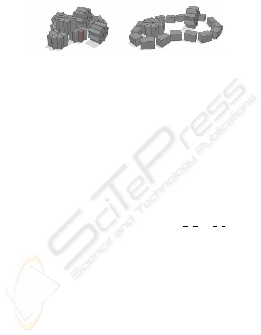
(a) (b)
Figure 1: Various configurations animated using the PGS–SM method. Configurations include composite rigid bodies, contact
constraints, and hinge joint constraints with joint limits.
Velocity based formulations suffer from none of these
problems, for this reason we use a velocity based for-
mulation for this paper. The approach we present
is based on reformulating the frictional problem as
a nonlinear complementarity problem. The result is
a slightly inaccurate model, with relatively few vari-
ables to solve for. This makes it advantageous in in-
teractive simulations from a performance viewpoint.
Our work is inspired by (Morales et al., 2008;
Arechavaleta et al., 2009). The novel contribution
consists of tailoring the ideas to suit the NCP formu-
lation, used for interactive rigid body dynamics. Fur-
ther, we present optimizations to the subspace method
to make the simulation fast enough for interactive us-
age. Prior work is limited to a linear complementarity
problem formulation, missing evaluation of the ideas
for general rigid body simulation. Application is lim-
ited to grasping, which is dominated by bilateral con-
straints and static friction. Here we evaluate with fo-
cus on both dynamic and static friction, as well as nor-
mal constraints.
2 THE NONLINEAR
COMPLEMENTARITY
PROBLEM FORMULATION
The frictional contact force problem can be stated as a
linear complementarity problem (LCP) (Stewart and
Trinkle, 1996). However, a different formulation is
used in interactive physical simulations, we will de-
rive this formulation. Without loss of generality, we
will only consider a single contact point. The focus of
this paper is on the contact force model, so the time
stepping scheme and matrix layouts are based on the
velocity-based formulation in (Erleben, 2007). We
have the time discretized Newton–Euler equations,
Mv −J
T
n
λ
n
− J
T
t
λ
t
= F, (1)
where J
n
is the Jacobian corresponding to normal
constraints and J
t
is the Jacobian corresponding to
the tangential contact impulses. M is the generalized
mass matrix and v is the generalized velocity vector.
We wish to solve for v in order to compute a posi-
tion update. For readability we have, without loss of
generality, abstracted the discretization details within
the Lagrange multipliers λ
n
, λ
t
and generalized ex-
ternal impulses F. Since the contact plane is two-
dimensional, we span this plane by two orthogonal
unit vectors, t
1
and t
2
. Any vector in this plane can be
written as a linear combination of these two vectors.
Thus, J
t
has only two rows corresponding to the two
directions. From (1) we can obtain the generalized
velocities,
v = M
−1
F + M
−1
J
T
n
λ
n
+ M
−1
J
T
t
λ
t
. (2)
Let the Lagrange multipliers λ =

λ
n
λ
T
t

T
and con-
tact Jacobian J =

J
n
J
t

T
, then we write the rela-
tive contact velocities y =

y
n
y
T
t

T
such that,
y = Jv = JM
−1
J
T
| {z }
A
λ + JM
−1
F
| {z }
b
. (3)
To compute the frictional component of the contact
impulse, we need a model of friction. We base our
model on Coulomb’s friction law. In one dimen-
sion, Coulomb’s friction law can be written as (Baraff,
1994),
y < 0 ⇒ λ
t
= µλ
n
, (4a)
y > 0 ⇒ λ
t
= −µλ
n
, (4b)
y = 0 ⇒ −µλ
n
≤ λ
t
≤ µλ
n
. (4c)
For the full contact problem, we split y into positive
and negative components,
y = y
+
− y
−
, (5)
where
y
+
≥ 0, y
−
≥ 0 and

y
+

T

y
−

= 0. (6)
For the frictional impulses, we define the bounds
−l
t
(λ) = u
t
(λ) = µλ
n
and for the normal impulse
PROJECTED GAUSS-SEIDEL SUBSPACE MINIMIZATION METHOD FOR INTERACTIVE RIGID BODY
DYNAMICS - Improving Animation Quality using a Projected Gauss-Seidel Subspace Minimization Method
39

l
n
(λ) = 0 and u
n
(λ) = ∞. Combining the bounds
with (4), (5) and (6), we reach the final nonlinear com-
plementarity problem (NCP) formulation,
y
+
− y
−
= Aλ + b, (7a)
y
+
≥ 0, (7b)
y
−
≥ 0, (7c)
u(λ) − λ ≥ 0, (7d)
λ − l(λ) ≥ 0, (7e)

y
+

T
(λ − l(λ)) = 0, (7f)

y
−

T
(u(λ) − λ) = 0, (7g)

y
+

T

y
−

= 0, (7h)
where l(λ) = [l
n
(λ) l
t
(λ)
T
]
T
and u(λ) =
[u
n
(λ) u
t
(λ)
T
]
T
. The advantage of the NCP
formulation is a much lower memory footprint
than for the LCP formulation. The disadvantage
is solving the friction problem as two decoupled
one-dimensional Coulomb friction models.
3 THE PROJECTED
GAUSS–SEIDEL METHOD
The following is a derivation of the PGS method for
solving the frictional contact force problem, stated as
the NCP (7). Using a minimum map reformulation,
the i
th
component of (7) can be written as
(Aλ + b)
i
= y
+
i
− y
−
i
, (8a)
min(λ
i
− l
i
, y
+
i
) = 0, (8b)
min(u
i
− λ
i
, y
−
i
) = 0. (8c)
where l
i
= l
i
(λ) and u
i
= u
i
(λ). Note, when y
−
i
> 0
we have y
+
i
= 0 which in turn means that λ
i
− l
i
≥ 0.
In this case, (8b) is equivalent to
min(λ
i
− l
i
, y
+
i
− y
−
i
) = −(y
−
)
i
. (9)
If y
−
i
= 0 then λ
i
− l
i
= 0 and complementarity con-
straint (8b) is trivially satisfied. Substituting (9) for
y
−
i
in (8c) yields,
min(u
i
− λ
i
, max(l
i
− λ
i
, −(y
+
− y
−
)
i
)) = 0. (10)
This is a more compact reformulation than (7) and
eliminates the need for auxiliary variables y
+
and y
−
.
By adding λ
i
we get a fixed point formulation
min(u
i
, max(l
i
, λ
i
− (Aλ + b)
i
)) = λ
i
. (11)
We introduce the splitting A = B − C and an iteration
index k. Then we define c
k
= b − Cλ
k
, l
k
= l(λ
k
) and
u
k
= u(λ
k
). Using this we have
min(u
k
i
, max(l
k
i
, (λ
k+1
− Bλ
k+1
− c
k
)
i
)) = λ
k+1
i
.
(12)
When lim
k→∞
λ
k
= λ
∗
then (12) is equivalent to (7).
Next we perform a case-by-case analysis. Three cases
are possible,
(λ
k+1
− Bλ
k+1
− c
k
)
i
< l
i
⇒ λ
k+1
i
= l
i
, (13a)
(λ
k+1
− Bλ
k+1
− c
k
)
i
> u
i
⇒ λ
k+1
i
= u
i
, (13b)
l
i
≤ (λ
k+1
− Bλ
k+1
− c
k
)
i
≤ u
i
⇒
λ
k+1
i
= (λ
k+1
−Bλ
k+1
− c
k
)
i
. (13c)
Case (13c) reduces to,
(Bλ
k+1
)
i
= −c
k
i
, (14)
which for a suitable choice of B and back substitution
of c
k
gives,
λ
k+1
i
= (B
−1
(Cλ
k
− b))
i
. (15)
Thus, our iterative splitting method becomes,
min(u
k
i
, max(l
k
i
, (B
−1
(Cλ
k
− b))
i
)) = λ
k+1
i
. (16)
This is termed a projection method. To realize this,
let λ
0
= B
−1
(Cλ
k
− b) then,
λ
k+1
= min(u
k
, max(l
k
, λ
0
)), (17)
is the (k + 1)
th
iterate obtained by projecting the
vector λ
0
onto the box given by l
k
and u
k
. Using
the splitting B = D + L and C = −U results in the
Projected Gauss–Seidel method. The resulting PGS
method (17) can be efficiently implemented as a for-
ward loop over all components and a component wise
projection. To our knowledge no known convergence
theorems exist for (16) in the case of variable bounds
l(λ) and u(λ). However, for fixed constant bounds the
formulation can be algebraically reduced to that of a
LCP formulation. In general, LCP formulations can
be shown to have linear convergence rate and unique
solutions, when A is symmetric positive definite (Cot-
tle et al., 1992). However, the A matrix equivalent
of our frictional contact model is positive symmetric
semi definite and uniqueness is no longer guaranteed,
but existence of solutions are (Cottle et al., 1992).
GRAPP 2010 - International Conference on Computer Graphics Theory and Applications
40

4 THE PROJECTED
GAUSS–SEIDEL SUBSPACE
MINIMIZATION METHOD
We will present a Projected Gauss–Seidel Subspace
Minimization (PGS–SM) method, specifically tai-
lored for the nonlinear complementarity problem for-
mulation of the contact force problem. Unlike previ-
ous work, which is limited to the linear complemen-
tarity problem formulation, our method is more gen-
eral and further specialized for interactive usage. The
PGS–SM method is an iterative method, each itera-
tion consisting of two phases. The first phase esti-
mates a set of active constraints, using the standard
PGS method. The second phase solves accurately for
the active constraints, potentially further reducing the
set of active constraints for the next iteration. In the
following we will describe the details of the PGS–SM
method.
4.1 Determining Index Sets
We define three index sets corresponding to our
choice of active constraints in (17)
L ≡
{
i|y
i
> 0
}
(18a)
U ≡
{
i|y
i
< 0
}
(18b)
A ≡
{
i|y
i
= 0
}
(18c)
assuming l
i
≤ 0 < u
i
for all i. The definition in (18) is
based on the y-vector. However, one may just as well
use the λ-vector, thus having
L ≡
{
i|λ
i
= l
i
}
(19a)
U ≡
{
i|λ
i
= u
i
}
(19b)
A ≡
{
i|l
i
< λ
i
< u
i
}
(19c)
When the PGS method terminates, we know λ is fea-
sible (although not the correct solution). However, y
may be infeasible due to the projection on λ made by
the PGS method. This votes in favor of using (19)
rather than (18). In our initial test trials, no hybrid or
mixed schemes seemed to be worth the effort. There-
fore, we use the classification defined in (19) for the
PGS–SM method.
4.2 Posing the Reduced Problem
Next we use a permutation of the indexes, creating the
imaginary partitioning of the system of linear equa-
tions (3)


y
A
y
L
y
U


=


A
A A
A
A L
A
AU
A
L A
A
L L
A
L U
A
UA
A
UL
A
UU




λ
A
λ
L
λ
U


+


b
A
b
L
b
U


.
(20)
Utilizing that ∀i ∈ A ⇒ y
i
= 0, as well as ∀i ∈ L ⇒
λ
i
= l
i
and ∀i ∈ U ⇒ λ
i
= u
i
, we get


0
y
L
y
U


=


A
A A
A
A L
A
AU
A
L A
A
L L
A
L U
A
UA
A
UL
A
UU




λ
A
l
L
u
U


+


b
A
b
L
b
U


.
(21)
To solve this system for y
L
, y
U
and λ
A
, we first com-
pute λ
A
from
A
A A
λ
A
= − (b
A
+ A
A L
l
L
+ A
AU
u
U
). (22)
Observe that A
A A
is a symmetric principal submatrix
of A. Knowing λ
A
, we can easily compute y
L
and
y
U
,
y
L
← A
L A
λ
A
+ A
L L
l
L
+ A
L U
u
U
+ b
L
, (23a)
y
U
← A
UA
λ
A
+ A
UL
l
L
+ A
UU
u
U
+ b
U
. (23b)
Finally, we verify that y
L
< 0, y
U
> 0 and l
A
≤ λ
A
≤
u
A
. If this holds, we have found a solution. Rather
than performing the tests explicitly, it is more simple
to perform a projection on the reduced problem
λ
A
← min(u
A
, max(l
A
, λ
A
)) (24)
We assemble the full solution λ ←

λ
T
A
l
T
L
u
T
U

T
,
before reestimating the index sets for the next itera-
tion. Observe that the projection on the reduced prob-
lem will either leave the active set unchanged or re-
duce it further.
4.3 The Complete Algorithm
The resulting algorithm can be outlined as
1 : while not convergence do
2 : λ ← run PGS for at least k
pgs
iterations
3 : if termination criteria is passed then
4 : return λ
5 : endif
6 : for k = 1 to k
sm
7 : L ≡
{
i|λ
i
= l
i
}
8 : U ≡
{
i|λ
i
= u
i
}
9 : A ≡
{
i|l
i
< λ
i
< u
i
}
10 : solve: A
A A
λ
A
= − (b
A
+ A
A L
l
L
+ A
AU
u
U
)
11 : y
L
← A
L A
λ
A
+ A
L L
l
L
+ A
L U
u
U
+ b
L
,
12 : y
U
← A
UA
λ
A
+ A
UL
l
L
+ A
UU
u
U
+ b
U
PROJECTED GAUSS-SEIDEL SUBSPACE MINIMIZATION METHOD FOR INTERACTIVE RIGID BODY
DYNAMICS - Improving Animation Quality using a Projected Gauss-Seidel Subspace Minimization Method
41

13 : update: (l, u)
14 : λ
A
← min(u
A
, max(l
A
, λ
A
))
15 : λ ←

λ
T
A
l
T
L
u
T
U

T
16 : if termination criteria is passed then
17 : return λ
18 : endif
19 : next k
20 : end while
An absolute termination criteria could be applied
ψ(λ) < ε
abs
(25)
where ψ is a merit function to the solution of (4), and
ε
abs
is a user specified value. An alternative termi-
nation criteria could be to monitor if the set A has
changed from previous iteration,
A(λ
k+1
) = A (λ
k
). (26)
A third termination criteria could be testing for stag-
nation
ψ(λ
k+1
) − ψ(λ
k
) < ψ(λ
k
)ε
rel
. (27)
for some user specified value ε
rel
> 0. Other merit-
functions could be used in place of ψ. Examples in-
clude natural merit functions of the Fischer reformu-
lation (Silcowitz et al., 2009) or the minimum map re-
formulation (Erleben and Ortiz, 2008). We prefer the
Fischer reformulation, as it seems to be more global
in the inclusion of boundary information (Billups,
1995). Finally, to ensure interactive performance, one
could use an absolute termination criteria on the num-
ber of iterations. Using such a criteria, the algorithm
may not perform iterations enough to reach an ac-
curate solution, we observed this behavior in a few
cases. To counter this, a fall back to the best iterate
found while iterating could be employed. This would
ensure that the PGS–SM method behaves no worse
than the PGS method would have done.
5 EXPERIMENTS
We have compared the PGS–SM method to the stan-
dard PGS method. For testing the PGS–SM method,
we have selected various test cases which we believe
to be challenging. The test cases are shown in Fig-
ure 2. The test cases include bilateral hinge joints
with joint limits, large mass-ratios, inclined plane se-
tups to provoke static friction handling, stacked con-
figurations of different sizes with both box and gear
geometries.
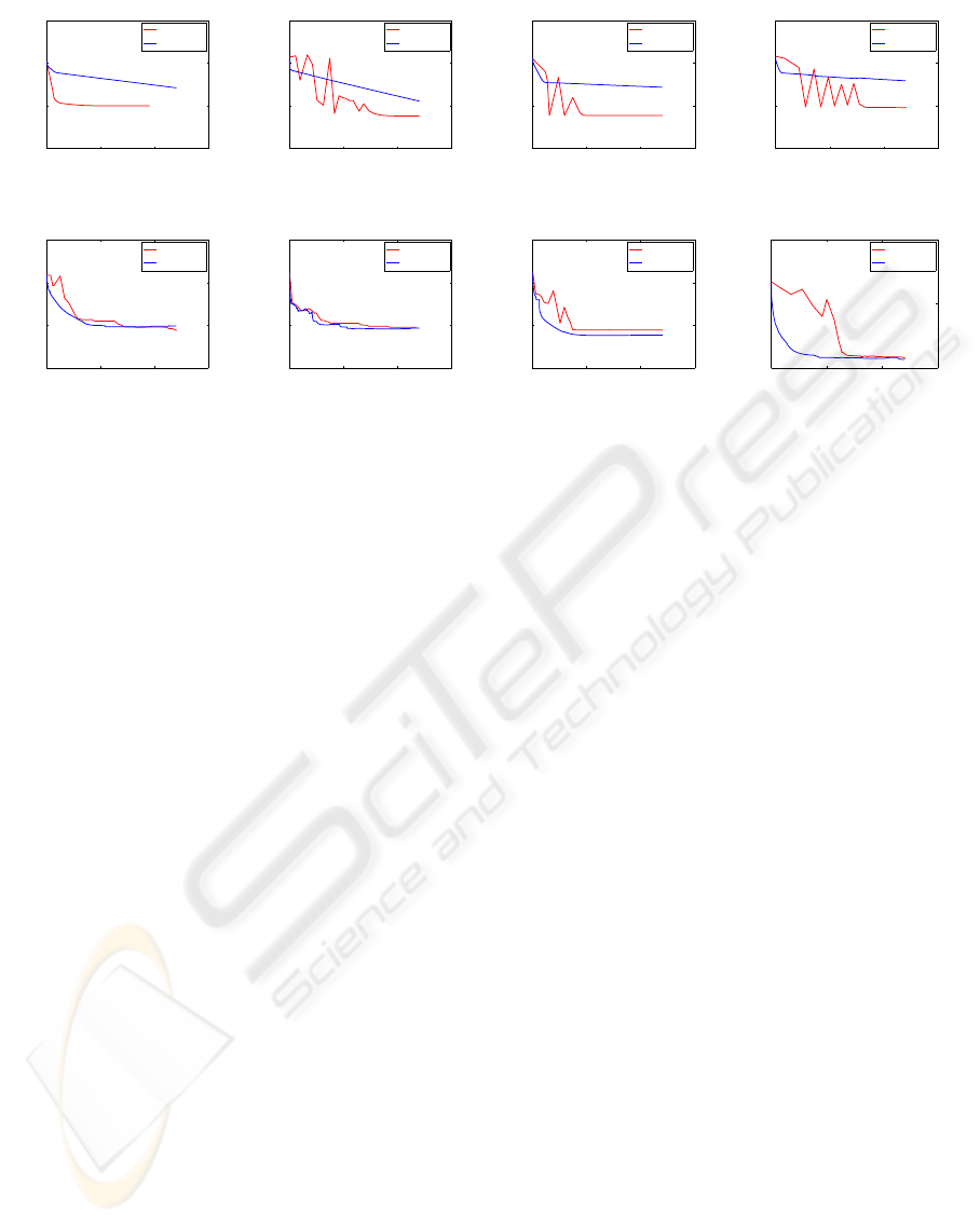
Convergence rates for all the test cases are shown
in Figure 3. In order to ease comparison, great care
is taken to measure the time usage of both methods in
units of PGS iterations.
For the tests, we use the iteration limits k
pgs
= 25
and k
sm
= 5. Further we use an error tolerance of
ε
abs
= 10
−15
. For the reduced problem we use a
non-preconditioned Conjugate Gradient (CG) method
with a maximum iteration count equal to the num-
ber of variables, and an error tolerance on the resid-
ual of ε
residual
= 10
−15
. The algorithms were imple-
mented in Java using JOGL, and the tests were run on
a Lenovo T61 2.0Ghz machine.
As observed in Figure 3, the PGS–SM method be-
haves rather well for small configurations and con-
figurations with joints. For larger configurations, we
obtain convergences similar to the PGS method.
The supplementary video shows interactive sim-
ulations of an articulated snake-like figure, compar-
ing the animation quality of the PGS–SM method to
the PGS method. All test cases run at interactive
frame rates, 25 fps or above. We have observed a
different quality in the motion simulated by the PGS–
SM method. It is our hypothesis that the PGS–SM
method seems to favor static friction over dynamic
friction. Our subjective impression is that the PGS–
SM method delivers a more plausible animation qual-
ity.
The presented algorithm is capable of very ac-
curate computations, compared to the PGS method.
However, we have observed problematic instances
where simulation blow-up was noticed. The simula-
tion blow-ups appear to occur regardless of how ac-
curate the subspace problem is solved. We observed
blow-ups even when using a singular value decompo-
sition pseudo inverse of the reduced problem (22).
In general, if bounds are fixed the problem reduces
to a LCP formulation. Applying a simple diagonaliza-
tion to the LCP, using an eigenvalue decomposition of
A, one can easily show that a solution to the problem
always exists when A is positive semi definite. How-
ever, when bounds are variable the nonlinear nature
of the problem makes it hard to say anything conclu-
sive about existence of a solution. The accuracy of
the system is thus clearly affected, when attempting
to solve a system that has no solution. The effect can
be observed in the behavior of the PGS method. By
increasing the number of iterations, the PGS method
will converge to a positive merit value. This indicates
convergence to a local minimizer of the merit func-
tion, and not a global minimizer.
GRAPP 2010 - International Conference on Computer Graphics Theory and Applications
42

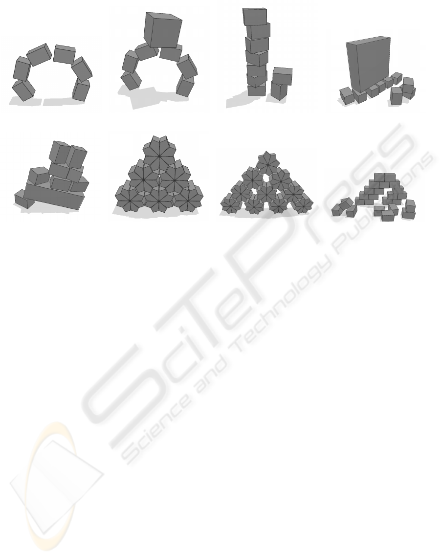
(a) (b) (c) (d)
(e) (f) (g) (h)
Figure 2: Illustrated test cases used for the PGS–SM method: (a) An arched snake composed of boxes and hinge joints with
limits, (b) A heavy box placed upon an arched snake, (c) A large stack of boxes of equal mass, (d) A heavy box resting on
lighter smaller boxes, (e) Boxes resting on an inclined surface resulting in static friction forces, (f) A small pyramid of gears,
(g) A medium-scale pyramid of gears, (h) A large configuration of boxes stacked in a friction inducing maner.
5.1 Stability Improvements
Stability can be improved by adding minor changes
to the presented algorithm. Such a change could be
the use of a relative termination criteria for the PGS
method similar to (27), thus forcing the method to it-
erate long enough to improve the estimate of the ac-
tive set. In our experience, this can be very beneficial
although it counteracts interactive performance.
Another strategy that seems to improve stability,
is to add numerical regularization to the sub-problem.
The matrix A
A A
is replaced with A
0
A A
= A
A A
+γI for
some positive scalar γ. The regularization makes A
0
A A
positive definite, which improves the performance of
the CG method. The result of the regularization is
observed as a damping in the contact forces. In our
opinion, it severely affects the realism of the simula-
tion but works quite robustly. In our experience, it
seems that one can get away with only dampening the
entries corresponding to friction forces.
Rather than regularizing the A-matrix, one could
regularize the bounds. We have experienced positive
results when applying a lazy evaluation of the bounds
inside the subspace solver loop. Thus, having slightly
relaxed bounds appear to add some freedom in reach-
ing proper friction forces. On the downside, it appears
to make the solver favor static friction solutions. We
leave this idea for future work.
One final variation we will mention, is the stag-
gered approach to the contact force problem. The
approach is conceptually similar to (Kaufman et al.,
2008). The idea is an iteration-like approach. First
solve for normal forces assuming fixed given friction
forces, and secondly solve for frictional forces assum-
ing fixed given normal forces. The advantage of the
staggered approach is that each normal and friction
sub-problem has constant bounds, thus the NCP for-
mulation is trivially reduced to a boxed MLCP, equiv-
alent to a LCP. Given the properties of the A-matrix
this guarantees solutions exist for the sub-problems.
However, whether the sequence of sub-problems will
converge in the staggered approach is hard to say. We
have not observed any conclusive results on using a
staggered approach.
6 CONCLUSIONS
A Projected Gauss–Seidel subspace minimization
(PGS–SM) method has been presented, evaluated
and compared to the Projected Gauss–Seidel (PGS)
method for interactive rigid body dynamics. The
PGS–SM method is stable for small sized configura-
tions with large mass ratios, static friction and bilat-
eral joints subject to limits. For medium and larger
sized configurations, the PGS–SM method deterio-
PROJECTED GAUSS-SEIDEL SUBSPACE MINIMIZATION METHOD FOR INTERACTIVE RIGID BODY
DYNAMICS - Improving Animation Quality using a Projected Gauss-Seidel Subspace Minimization Method
43

0 500 1000 1500
10
−40
10
−20
10
0
10
20
Arched Snake
PGS iterations
Ψ(λ
k
)
PGS−SM
PGS
(a)
0 500 1000 1500
10
−10
10
−5
10
0
10
5
Heavy Box On Arched Snake
PGS iterations
Ψ(λ
k
)
PGS−SM
PGS
(b)
0 500 1000 1500
10
−20
10
−10
10
0
10
10
Large Stack of Boxes
PGS iterations
Ψ(λ
k
)
PGS−SM
PGS
(c)
0 500 1000 1500
10
−20
10
−10
10
0
10
10
Heavy Box Resting On Light Boxes
PGS iterations
Ψ(λ
k
)
PGS−SM
PGS
(d)
0 500 1000 1500
10
−10
10
−5
10
0
10
5
Boxes Resting On Inclined Surface
PGS iterations
Ψ(λ
k
)
PGS−SM
PGS
(e)
0 500 1000 1500
10
−10
10
−5
10
0
10
5
Small Pyramid of Gears
PGS iterations
Ψ(λ
k
)
PGS−SM
PGS
(f)
0 500 1000 1500
10
−10
10
−5
10
0
10
5
Medium Pyramid Of Gears
PGS iterations
Ψ(λ
k
)
PGS−SM
PGS
(g)
0 500 1000 1500
10
−5
10
0
10
5
Friction Dependant Structure
PGS iterations
Ψ(λ
k
)
PGS−SM
PGS
(h)
Figure 3: Corresponding convergence plots for the test cases in Figure 2. Observe the jaggyness in the PGS–SM plots in (b),
(c), (d), and (g). The spikes indicates that the PGS–SM method guessed a wrong active set. This can cause the merit function
to rise abruptly. The ψ funciton is the Fischer function from (Silcowitz et al., 2009).
rates into convergence behavior similar to the PGS
method. Still, the PGS–SM method shows qualita-
tively different appearance in the simulations. For
larger configurations, the PGS–SM method may be
subject to simulation instability. In our opinion, our
investigations indicate a more fundamental problem
with the nonlinear complementarity problem (NCP)
formulation of the contact force problem. We specu-
late that existence of solution is vital when accurate
computations are performed. The minimum norm na-
ture of the PGS method handles such cases robustly,
although not very accurately.
Future work may include investigation into the na-
ture of the NCP formulation, addressing existence of
solutions. A more practical viewpoint would be ex-
ploring various iterative solvers for the reduced prob-
lem, as well as regularization ideas for the NCP for-
mulation. In particular, we find the lazy evaluation of
friction bounds appealing.
REFERENCES
Anitescu, M. and Potra, F. A. (1997). Formulating dy-
namic multi-rigid-body contact problems with friction
as solvable linear complementarity problems. Nonlin-
ear Dynamics. An International Journal of Nonlinear
Dynamics and Chaos in Engineering Systems.
Arechavaleta, G., E.Lopez-Damian, and Morales, J. (2009).
On the use of iterative lcp solvers for dry frictional
contacts in grasping. In International Conference on
Advanced Robotics 2009, ICAR 2009.
Baraff, D. (1994). Fast contact force computation for non-
penetrating rigid bodies. In SIGGRAPH ’94: Pro-
ceedings of the 21st annual conference on Computer
graphics and interactive techniques.
Billups, S. C. (1995). Algorithms for complementarity prob-
lems and generalized equations. PhD thesis, Univer-
sity of Wisconsin at Madison.
Cottle, R., Pang, J.-S., and Stone, R. E. (1992). The Linear
Complementarity Problem. Academic Press.
Erleben, K. (2007). Velocity-based shock propagation for
multibody dynamics animation. ACM Trans. Graph.,
26(2).
Erleben, K. and Ortiz, R. (2008). A Non-smooth Newton
Method for Multibody Dynamics. In American Insti-
tute of Physics Conference Series.
Featherstone, R. (1998). Robot Dynamics Algorithms.
Kluwer Academic Publishers, second printing edition.
Guendelman, E., Bridson, R., and Fedkiw, R. (2003). Non-
convex rigid bodies with stacking. ACM Trans. Graph.
Hahn, J. K. (1988). Realistic animation of rigid bodies. In
SIGGRAPH ’88: Proceedings of the 15th annual con-
ference on Computer graphics and interactive tech-
niques.
Kaufman, D. M., Sueda, S., James, D. L., and Pai, D. K.
(2008). Staggered projections for frictional contact in
multibody systems. ACM Trans. Graph., 27(5).
Milenkovic, V. J. and Schmidl, H. (2004). A fast impulsive
contact suite for rigid body simulation. IEEE Transac-
tions on Visualization and Computer Graphics, 10(2).
Mirtich, B. V. (1996). Impulse-based dynamic simulation
of rigid body systems. PhD thesis, University of Cali-
fornia, Berkeley.
Moore, M. and Wilhelms, J. (1988). Collision detection
and response for computer animation. In SIGGRAPH
GRAPP 2010 - International Conference on Computer Graphics Theory and Applications
44

’88: Proceedings of the 15th annual conference on
Computer graphics and interactive techniques.
Morales, J. L., Nocedal, J., and Smelyanskiy, M. (2008).
An algorithm for the fast solution of symmetric linear
complementarity problems. Numer. Math., 111(2).
O’Sullivan, C., Dingliana, J., Giang, T., and Kaiser, M. K.
(2003). Evaluating the visual fidelity of physically
based animations. ACM Trans. Graph., 22(3).
Redon, S., Kheddar, A., and Coquillart, S. (2003). Gauss
least constraints principle and rigid body simulations.
In In proceedings of IEEE International Conference
on Robotics and Automation.
Silcowitz, M., Niebe, S., and Erleben, K. (2009). Nons-
mooth Newton Method for Fischer Function Refor-
mulation of Contact Force Problems for Interactive
Rigid Body Simulation. In VRIPHYS 09: Sixth Work-
shop in Virtual Reality Interactions and Physical Sim-
ulations, pages 105–114. Eurographics Association.
Stewart, D. E. (2000). Rigid-body dynamics with friction
and impact. SIAM Review.
Stewart, D. E. and Trinkle, J. C. (1996). An implicit time-
stepping scheme for rigid body dynamics with in-
elastic collisions and coulomb friction. International
Journal of Numerical Methods in Engineering.
Trinkle, J. C., Tzitzoutis, J., and Pang, J.-S. (2001). Dy-
namic multi-rigid-body systems with concurrent dis-
tributed contacts: Theory and examples. Philosophi-
cal Trans. on Mathematical, Physical, and Engineer-
ing Sciences.
PROJECTED GAUSS-SEIDEL SUBSPACE MINIMIZATION METHOD FOR INTERACTIVE RIGID BODY
DYNAMICS - Improving Animation Quality using a Projected Gauss-Seidel Subspace Minimization Method
45