SETTING GRAPH CUT WEIGHTS FOR AUTOMATIC

FOREGROUND EXTRACTION IN WOOD LOG IMAGES

Enrico Gutzeit, Stephan Ohl, Arjan Kuijper, Joerg Voskamp and Bodo Urban

Fraunhofer Institute for Computer Graphics Research IGD, Joachim-Jungius-Str. 11, 18059 Rostock, Germany

Keywords:

Image segmentation, Graph cuts, Foreground extraction, Weight setting.

Abstract:

The automatic extraction of foreground objects from the background is a well known problem. Much research

has been done to solve the foreground/background segmentation with graph cuts. The major challenge is

to determine the weights of the graph in order to obtain a good segmentation. In this paper we address

this problem with a focus on the automatic segmentation of wood logs. We introduce a new solution to get

information about foreground and background. This information is used to set the weights of the graph cut

method. We compare four different methods to set these weights and show that the best results are obtained

with our novel method, which is based on density estimation.

1 INTRODUCTION

Graph-cut based segmentation techniques are a very

powerful tool in image segmentation. In interactive

image analysis, e.g. in medical imaging (F. Malmberg

and Borgefors, 2009), it is possible to get a good seg-

mentation with only a few reﬁnements. In a fully au-

tomatic system there is no possibility for reﬁnements

and so the problem of initialization of the graph-cut

algorithm, mainly setting the weights for the graph, is

a difﬁcult problem. In this paper the problem is es-

pecially addressed to automatically and soundly seg-

ment wood log images.

The volume of wood and the sizes of the logs

are important factors of commercial and logistic pro-

cesses in timber industry. There are different methods

to measure the amount of wood. Most reliable tech-

niques are laser scanning methods or wood weighing

for volume analysis. These methods, however, are

mainly used in factories since they are relatively dif-

ﬁcult to apply. In forests estimations are used often.

After logs have been cut they are piled up onto stacks.

The amount of cut wood is then estimated from the

front side of the stack. Furthermore, the distribution

of log diameters is estimated by visual judgment only.

It is described by a constant because measuring the di-

ameter of each log is impossible in practice.

Our aim is to use computer vision methods to

make these front side measurements faster and more

reliable. Separating the log cut surfaces from the

background leads to the well known problem of bi-

nary image segmentation. A robust automatic binary

segmentation allows more accurate volume estima-

tion techniques than the manual one described brieﬂy

above. The imaging devices we use are mobile phone

cameras as these are lightweight common place de-

vices. On the other hand, their optics incorporate

some trade-offs on image quality. Furthermore, we

restrict ourselves to images taken from frontal posi-

tions.

The contribution of this paper is a methodology

for automatic and robust foreground / background

segmentation of these low quality wood log images.

We use a min-cut/max-ﬂow graph-cut algorithm in

conjunction with a kd-tree accelerated density estima-

tion. Our novel density estimation improves current

approaches with respect to robustness and is relatively

simple to implement, which we call KD-NN in the

following. The methodology is split into two parts.

First, we make use of some properties of the image

structure to initiate models in color space. Second,

we used them to yield the ﬁnal segmentation. The

graph-cut algorithm is used in both steps.

2 RELATED WORK

Our speciﬁc application has been considered in imag-

ing barely. (Fink, 2004) describes classical vision al-

gorithms and active contours to ﬁnd the log cut sur-

faces. The proposed procedure is only half automatic

Gutzeit E., Ohl S., Kuijper A., Voskamp J. and Urban B. (2010).

SETTING GRAPH CUT WEIGHTS FOR AUTOMATIC FOREGROUND EXTRACTION IN WOOD LOG IMAGES.

In Proceedings of the International Conference on Computer Vision Theory and Applications, pages 60-67

DOI: 10.5220/0002831000600067

 SciTePress

and makes a lot of assumptions about the type of

wood, the lighting conditions and the image quality.

The photos of the stack of wood are taken in a con-

trolled environment which makes the proposed algo-

rithms useless in our scenario.

In computer vision there is a variety of approaches

to tackle the binary segmentation problem (Jaehne,

2005). However, when it comes to stable and fully

automatic segmentation of natural images, things are

getting complicated. Normalized Cuts (Shi and Ma-

lik, 2000) are used to ﬁnd a reasonable partition of the

image. But these kinds of algorithms are optimized in

order to solve the grouping problem in vision.

Instead, we focused on a quite popular binary seg-

mentation framework from the ﬁelds of combinatorial

optimization. Hereby, a graph-cut results from solv-

ing for the maximum ﬂow (Boykov and Jolly, 2001).

The corresponding minimum cut then describes the

resulting partition of the image. There are algorithms

that are optimized for grid-graphs (Boykov and Kol-

mogorov, 2004) and provide a feasible solution in a

few seconds, even for megapixel sized images.

There are different approaches to set the weights

of the graph. The weights between two adjacent ver-

tices are set often by using some metric like the eu-

clidian for instance. While ﬁnding a pixel to pixel

distance is straight forward, existing algorithms differ

in setting the weights for the remaining edges to the

source and the sink node. A good and practical solu-

tion for gray scaled images is the usage of a histogram

which describes the two necessary distributions for

binary segmentation (Boykov and Jolly, 2001). In the

case of RGB images, it is more challenging to ﬁnd

a model for the two distributions. In (C. Rothar and

Blake, 2004) a Gaussian Mixture Model (GMM) is

used for description. However, the method deals with

interactive segmentation. It is derived from (Orchard

and Bouman, 1991).

We implemented this GMM method and found it

unstable. The method is quite prone to outliers. In

interactive segmentation, this is not so important be-

cause the model can be changed quickly. But this does

not meet our requirements. Instead, in our compari-

son we replaced the method for estimating the GMMs

by the Expectation Maximization algorithm.

3 PROBLEM DISCUSSION

The volume especially the solid cubic meter of a stack

of wood is simple computable via a multiplication of

the area of the log cut surfaces with the depth. The

depth per stack of wood is known, but not the wood

surfaces. To determine the wood area from images,

the stack of wood must be taken from a frontal posi-

tion, whereby the log cut surfaces must be visible (see

ﬁgure 2).

To obtain the area of wood the image must ﬁrst

transform into a real coordinate system, so that every

pixel has the same area in real square meter. Secondly,

a stack of wood often doesn’t ﬁt into a single image.

Due to this problem more images must be taken from

one stack of wood and be stitched together. Thirdly,

a segmentation is required to separate the wood and

non-wood pixel. How to transform the images and

stitch them together is beyond the scope of this paper.

Therefore, we here only address the third problem, the

segmentation.

The objective is to separate automatically and

soundly the log cut surfaces from different images.

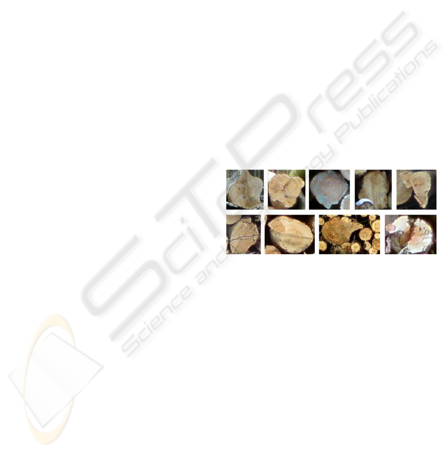
Log cut surfaces of a stack of wood in praxis vary

in shape and color. The shape of an log cut surface

seems to be a circle or an ellipse, but that is not ever

given in praxis (see ﬁgure 1). Therefore a shape ﬁnd-

ing technique, e.g. ellipse ﬁtting, cannot be applied.

Furthermore the color from one stack of wood to an-

other is different and dependent on the wood type,

whereby no general color matching is appropriate.

Figure 1: Logs with different shape and color.

Logs have a certain self-similarity, but in a dif-

ferent degree. Hence the usage of simple region

based methods, e.g. watershed or split and merge,

lead to the well known problem of under- or over-

segmentation. In summary, there is no exact color

or shape for all logs usable, but for one single stack

of wood the color is mostly similar and the gradients

between logs and non logs are often high.

For this reason we extract color information from

the image ﬁrst and use this to segment the image. To

use both characteristics of local gradient and global

color a graph-cut approach is used.

4 OUR APPROACH

For our approach we require some general restrictions

on the image acquisition to have some context infor-

mation. First, the image needs to be taken from a

SETTING GRAPH CUT WEIGHTS FOR AUTOMATIC FOREGROUND EXTRACTION INWOOD LOG IMAGES

frontal position as mentioned earlier and the stack of

wood has to be in the center. Second, the upper and

lower area of the image must not contain log cut sur-

faces. This is realized in common praxis because a

stack of wood has a limited height (see also ﬁgure 2).

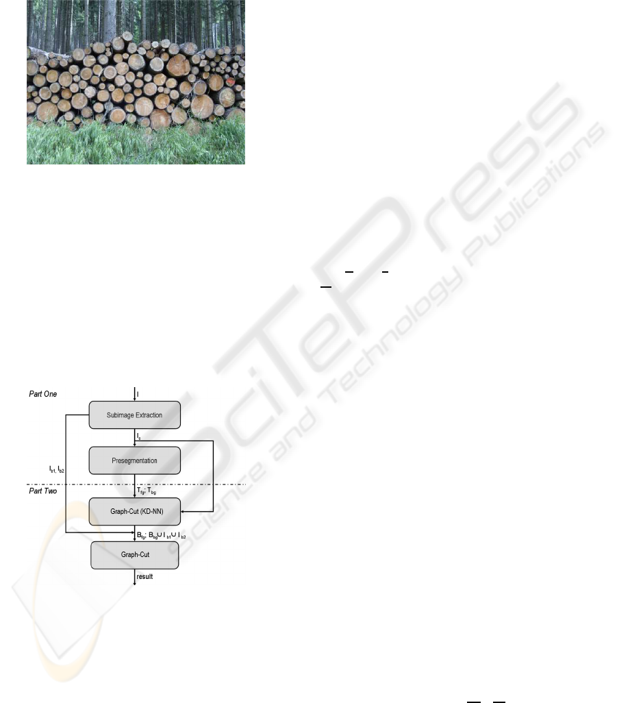
Figure 2: A sample image of a stack of wood.

In the following, the image part that represents

the log cut surfaces is called foreground and the re-

maining areas are called background. This follows

the common naming conventions in graph-cut papers.

The segmentation is generally split into two main

parts (see ﬁgure 3). In step one a region in the center

of the input image is used to extract information about

the log cut surfaces and the darker regions in between.

In this step a number of properties and a ﬁrst graph-

cut with our novel KD-NN to set the graph weights

are used.

Figure 3: The two parts of the segmentation procedure.

Additionally, one subimage from the bottom and

one from the top are used to gain information about

the background. Both subimages are needed because

they represent characteristics of quite different parts

of the image, e.g. sky, forest, soil, snow or grass.

This information is used together with the back-

ground characteristics to apply graph-cut a second

time to the whole input image, but this time with dif-

ferent weight setting algorithms for later comparison.

Background characteristics means the objects in front

of and behind the stack of wood. All steps are de-

scribed in detail in the following sections.

4.1 Our Novel Approach for Fore- and

Background Extraction

The aim of the ﬁrst part of the segmentation is to ﬁnd

a ﬁrst estimate for the foreground (log cut surfaces)

and background color models. These models are nec-

essary for the graph-cut algorithm to accurately seg-

ment the log cut surfaces. The following description

is also illustrated in ﬁgure 3.

Let I denote the input image of size m×n where m

is the height and n the width. We extract three subim-

ages from I. First, we extract a subimage I

from the

center region. The other two subimages, I

and I

are extracted from the top and bottom of I respec-

tively. Due to the constraints in image acquisition,

contains log cut surfaces only and the shadowed re-

gions in between whereas I

and I

contain regions

to be classiﬁed as background. We chose I

to be of

size ⌊

⌋ × ⌊

⌋. I

and I

are horizontal bars of size

⌊

⌋ × n. Our experiments have proven these dimen-

sions reasonable.

Whereas the pixels of I

and I

can directly be

used for the background model we need to segment

into foreground and background pixels. We do this

by using a stable novel method which is described in

detail in the following.

Segmenting I

is much easier than the segmenta-

tion of I because the difference in luminance between

the log cut surfaces and shadowed regions in between

is very strong. Nevertheless, muddy logs, different

types of wood and leaves are disturbing factors.

Hence, for a stable segmentation we use the inter-

section of two binary threshold segmentations where

each of these is performed in another color space. The

V-channel from the HSV color space is thresholded

directly. In RGB color space we use the observation

that wood surfaces often contain a strong yellow com-

ponent. Therefore, we extract Y from the RGB image

using the following equation pixel wise.

Y = max(min(R− B, G− B), 0) (1)

Both channels V and Y are automatically thresholded

by using the method in (Otsu, 1979). The resulting

binary images are V

and Y

. The intersection of both

= V

∩Y

(2)

= V

∩Y

(3)

results in a trimap T = (T

, T

unknown

). T

is the

foreground, T

is the background and T

unknown

are

pixels of which it is not known, if they belong to

VISAPP 2010 - International Conference on Computer Vision Theory and Applications

the foreground or the background. T

unknown

is ex-

panded further by morphological operators to ensure

deﬁnitely a clean segmentation.

To get a more accurate binary segmentation of I

a ﬁrst graph-cut segmentation is used. The pixel sets

and T

are used to build the foreground and back-

ground model. The result is a binary segmentation

B = (B

, B

). For the ﬁnal segmentation a second

graph cut is applied to I. The pixel set to describe the

foreground is B

. The background model is built by

using the pixel set union B

∪ I

4.2 Graph-Cut and Weight Setting

Graph based image segmentation methods represent

the problem in terms of a graph G = (V, E). The

graph consists of a set of nodes v ∈ V and a set of

weighted edges e ∈ E connecting them. In an image

each node corresponds to a pixel which is connected

to its 4 neighbors. Additionally there are two special

nodes called terminals (sink and source), which rep-

resent foreground and background. Each node has a

link to either of the terminals.

In the following let w

be the weights of the edges

connecting pixels and terminals and let w

be the

weights of inter pixel edges. We assume that all

weights w

, w

for the graph are in the interval [0, 1].

A vector in feature space (RGB color space) is de-

noted by x.

For setting the w

, we applied the following for-

mula, whereby i and j indicate adjacent graph nodes.

= 1− e

−α∗kx

−x

(4)

We used the Manhattan Metric because it is a little

faster than the Euclidian Metric and the difference in

segmentation results was negligible for our images.

A higher choice for the value of the free parameters α

leads to more similarity between two feature vectors.

For setting the w

to the terminal nodes we imple-

mented four different feature space analysis methods,

each of which is described in detail in the following

subsections. In every case we built two models, one

for the foreground and one for the background respec-

tively. We did not introduce indices in the formulas to

keep the notation uncluttered.

After having set all weights, the min-cut/max-ﬂow

algorithm from (Boykov and Kolmogorov, 2004) is

applied. The results of each of the four following

feature space analysis methods are presented and dis-

cussed in chapter 5.

In the following we describe four different meth-

ods to determine w

by using the foreground pixels

and the background pixels B

. Afterward the re-

sults will be present and compared.

4.2.1 Histogram Probability

A simple method to determine a probability is to use

a histogram. We used a 3D histogram to approx-

imate the distribution of the foreground and back-

ground over the color space. One bin of the histogram

represent a probability p

. The probability can be

used to determine w

. To reduce noise, we scale the

histogram with the factor hs ∈ [0, 1], which is experi-

mentally set and used for comparison. The number of

bins per color channel in our case is calculated with

⌊256∗hs⌋. Another problem of histograms are peaks,

which lead to many low probabilities. Peaks in our

case arise from many pixel with the same color in B

or B

. To get a suitable weight the histogram is nor-

malized ﬁrst, so that the maximal bin has a probabil-

ity of 1. Afterward, the weights are determined by the

following equation, which get the best results in our

experiments.

= 1− e

−β∗sum

∗p

(5)

The sum

indicates the sum of all bins, p

the bin

value and so the probability of the corresponding

pixel and β is a free parameter.

4.2.2 K-Mean Clustering

Clustering is a common used method to groupingsim-

ilar points into different clusters. K-Mean is a simple

clustering algorithm and is often used to cluster the

color space. In our case we are applied K-Mean to

cluster the background and foreground pixels. The

results are k cluster with the mean m

, whereby i ∈

{1, ..., k}. To determine the weights different ways are

possible. One possibility is to ﬁnd the nearest cluster

mean m

, calculate the distance d

min

between the pixel

and m

and directly determine the weight. Another

way is to determine the weights using the average of

all distances to all cluster means m

. Additionally the

amount of pixels per cluster can also be included for

weight computation. We experimentally found out,

that the best segmentation results are created by using

the euclidian distance to one cluster mean and the free

parameter γ by

= 1− e

−γ∗d

min

(6)

4.2.3 Gaussian Mixture Models

A Gaussian Mixture Models (GMM) is a compact

way to describe a density function. It may be seen

as a generalization of K-Means Clustering. The stan-

dard way to ﬁnd the mean vectors and covariance ma-

trices of a GMM of K components is the Expectation

Maximization Algorithm. To speed up learning we

additionally sampled from our learning data.

SETTING GRAPH CUT WEIGHTS FOR AUTOMATIC FOREGROUND EXTRACTION INWOOD LOG IMAGES

When predicting from the model we can not take

the density function values directly to initialize the

weights of the graph. The reason therefor are very

small probability values and sharply peaked gaussian

components. Instead, we used it in a similar fashion

like the K-Mean Clustering. We left the normaliza-

tion factors out in the prediction phase, so our model

reduces to

∑

k=1

∗ exp(−

(µ

− x)

−1

(µ

− x)). (7)

The π

sum up to 1. That means the weights w

will lie in [0, 1]. The difference to the cluster centers

is anisotropic, whereby the simple K-Means approach

leads to isotropic differences. We notate this method

with EM-GMM in the following.

4.2.4 Our Novel Density Estimation by Nearest

Neighborhood

Our novel method is based on density estimation by

using a kd-tree, which we named KD-NN. To set the

weights to source and sink node we use two kd-tree

based models. The kd-trees contain all selected pix-

els and the associated values. One contains the fore-

ground and one the background pixels. So all infor-

mation is stored and used to set the weights in a later

step by using NN. The used model is similar to a pho-

ton map in (Jensen, 2001). A photon map contains

photons, our contains pixels. Both are used for den-

sity estimation. For fast NN search a balanced kd-tree

is needed. We use a data driven kd-tree and save a

pixel in relation to the color value. Each node of the

tree splits the color space by one dimension, stores

the position in color space and the number of pixels.

We built a balanced kd-tree (Jensen, 2001). Building

a kd-tree in this way is a O(n∗ logn) operation.

Similar to (Felzenszwalb, 2004) nearest neighbor-

hoods are involved. The NN are used for density esti-

mation and setting the region weights w

. Especially

for every graph node v the corresponding density in

color space within a sphere is used.

The ﬁrst step is to determine the density in rela-

tion to all pixels in the kd-tree. Hence, the number

of pixels p

all

in the kd-tree and the volume of the

color space are used to calculate an overall density

all

. In our case, we use the RGB color space, where

R, G, B ∈ [0, 255], and compute the density

all

255

. (8)

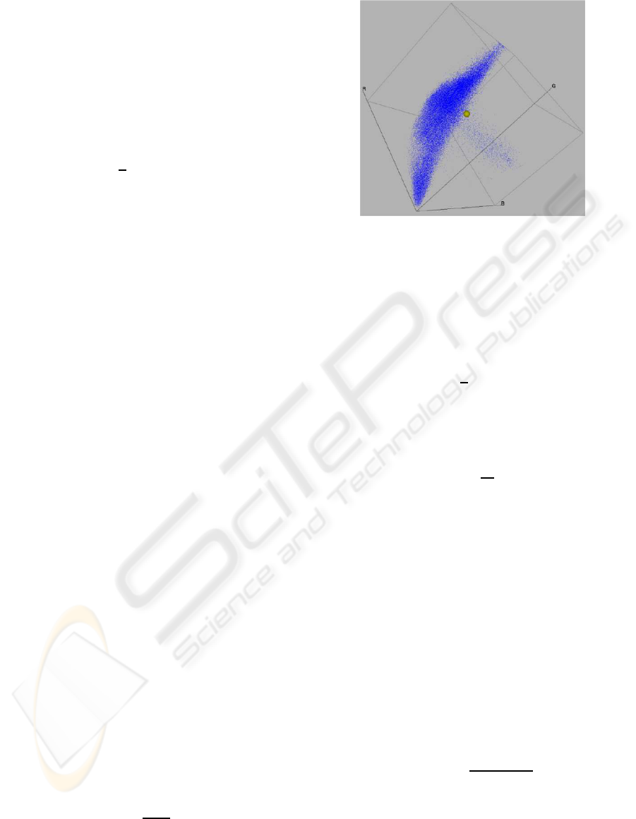
We estimate the density for every v by using its

sphere environment (see ﬁgure 4). The number of

pixels within this sphere with a predeﬁned radius r is

Figure 4: The pixels of the log cut surfaces are visualized as

points in RGB color space. The yellow sphere demonstrates

the search environment for the density estimation. Also,

there is a number of outliers.

searched in the kd-tree. The NN search in a balanced

kd-tree is an O(log(n)) operation (Samet, 2006). The

volume of the search sphere v

∗ π∗ r

. (9)

The density ρ

within the sphere environment is

estimated by the number of found pixels p

. It is used

for the weight calculation in the following section.

(10)

The setting of w

is done by the density ρ

. How-

ever, the number of pixels in one kd-tree and hence

all

is different and depends on the foreground and

background pixels. Hence, we use the overall density

all

to determine a factor s, which is taken for weight

computation.

The idea is to map the overall density ρ

all

, which

is also the mean density from the spheres in all possi-

ble positions, to a deﬁned weight w

. So, if the mean

density is found, the weight w

will be equal to w

In addition, a greater density than ρ

all

must produce a

high weight and a lower density a low weight, which

all must be in the interval [0, 1]. Therefore, the factor

is determinated by the following equation.

= 1 − e

−ρ

all

∗s

(11)

s =

ln(1− w

)

−ρ

all

(12)

Finally, the region weights are estimated by the den-

sity in the search sphere and the predetermined factor

s by

= e

−ρ

∗s

. (13)

VISAPP 2010 - International Conference on Computer Vision Theory and Applications

5 RESULTS

We tested our approach on images taken by employ-

ees from forestry. Due to the image acquisition with a

mobile phone, our tested input images are jpeg com-

pressed with maximal resolution of 2048× 1536 pix-

els. In our application we implemented the weight

computation in four different ways as described be-

fore. All methods determine the edge weights w

speciﬁed in 4.2 but differ in the calculation of the w

In our novel approach the graph-cut is processing

twice. To compare the different methods the same

weight setting for graph-cut in the presegmentation

is used. Hence the same conditions, especially the

same foreground B

and background pixels B

, are

given for the second graph-cut. We generally used

the best method for setting the weights our KD-NN

for the graph cut segmentation as evaluated later. In

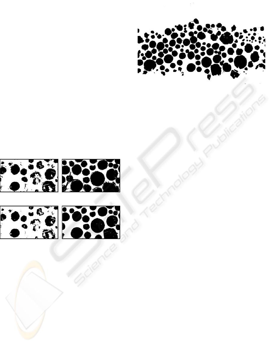
ﬁgure 5 and 6 the different states of the presegmenta-

tion and the ﬁnal result of the input image (ﬁgure 2)

are shown. Thereby the image quality improves over

the consecutive steps.

(a) (b)

Figure 5: The different steps of the presegmented center im-

age are shown. Image (a) shows the thresholded modiﬁed

Y-channel, (b) the thresholded V-channel and (c) the inter-

section of (a) and (b). In Image (d) the result of the ﬁrst

graph cut with KD-NN is shown.

For the comparison of the different weight set-

ting methods including our novel KD-NN from sec-

tion 4.2, we performed a ground truth test. Therefore

71 very different sample images with wood logs were

marked and the difference to the segmentation result

were measured as shown in ﬁgure 7. We experimen-

tally choose the best parameter to determine w

. The

weights created with the histogram were calculated

with β = 1000. For K-Mean γ was set to 0.02 and for

our KD-NN w

= 0.5 and r = 2.5 were used. For all

methods we used α = 0.0005 for w

.The simple RGB

color space, where R, G, B ∈ [0, 255] was used in all

methods.

Figure 6: The ﬁnal segmentation of the second graph-cut

run with KD-NN by using the presegmented center image,

which is shown in ﬁgure 5.

We measured the difference to the ground truth by

three values. The ﬁrst is the percent amount of too lit-

tle segmented pixels, which are notated as false neg-

ative. The second is the percent amount of too much

segmented pixels and the third the sum of them, which

is also the general error in the segmentation. This all

is in relate to the number of pixels in the image. Fur-

thermore we calculate the standard derivation of the

values. The table 1 shows the three measured values

for the different methods.

In table 1 it can be seen, that our KD-NN leads

to the least general segmentation error. The K-Mean

with eight clusters, whereby each cluster is initial po-

sitioned in one corner of the color cube, lead to similar

results. The Histogram generally gives the worst re-

sults and the EM-GMM is a little better. K-Mean and

KD-NN are the best methods for setting the weights

in our application, whereby KD-NN performs slightly

better.

6 CONCLUSIONS AND FUTURE

WORK

We present a novel method to segment accurately log

cut surfaces in pictures taken from a stack of wood

by smart phone cameras using the min-cut/maxﬂow

framework. If certain restrictions on the image acqui-

sition are made, the described approach is robust un-

der different lighting conditions and cut surface col-

ors. Robustness stems from our new, relatively simple

and easy to implement density estimation. We com-

pared our method with other approached and showed

that we mostly outperformed them. Our method lead

to similar results as K-Mean clustering of the color

space. However, our method is faster because of the

kd-tree we are using. It is also robuster against out-

liers, which can be a problem using K-Means cluster-

SETTING GRAPH CUT WEIGHTS FOR AUTOMATIC FOREGROUND EXTRACTION INWOOD LOG IMAGES

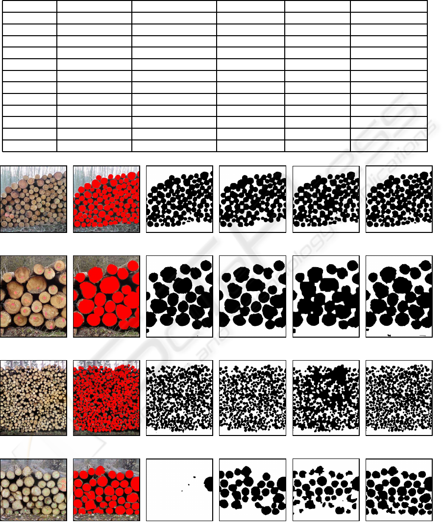
Table 1: The measured difference to the ground trues for all methods are shown here. The standard derivations are represented

in brackets.

Method number of bins amount of cluster false negative false positive false segmented

Histogram 16 - 14, 62(17, 04) 11, 29(14, 36) 25, 91(14, 74)

Histogram 32 - 7, 8(12, 33) 8, 95(9, 94) 16, 75(12)

Histogram 64 - 3, 45(5, 52) 7, 85(8, 32) 11, 3(8, 23)

Histogram 128 - 2, 62(3, 38) 7, 72(8, 12) 10, 34(7, 57)

Histogram 256 - 2, 73(2, 45) 7, 73(7, 99) 10, 46(7, 2)

EM-GMM - 2 4, 28(4, 44) 4, 87(4, 46) 9, 15(4, 64)

EM-GMM - 4 4, 02(4, 69) 5, 23(4, 31) 9, 25(4, 92)

EM-GMM - 8 3, 72(3, 91) 5, 57(4, 59) 9, 29(4, 67)

EM-GMM - 12 3, 75(3, 94) 5, 75(4, 91) 9, 5(4, 87)

EM-GMM - 16 3, 63(3, 87) 5, 9(4, 9) 9, 53(4, 75)

K-Mean - 8 3, 69(3, 93) 4, 29(3, 1) 7, 98(4, 27)

KD-NN - - 2, 38(3, 03) 5, 35(3, 67) 7, 73(3, 94)

(a) Sample Image (b) Ground Truth (c) Histogram (d) K-Mean (e) EM-GMM (f) KD-NN

(g) Sample Image (h) Ground Truth (i) Histogram (j) K-Mean (k) EM-GMM (l) KD-NN

(m) Sample Image (n) Ground Truth (o) Histogram (p) K-Mean (q) EM-GMM (r) KD-NN

(s) Sample Image (t) Ground Truth (u) Histogram (v) K-Mean (w) EM-GMM (x) KD-NN

Figure 7: Segmentation of four sample images (a),(g),(m),(s), the ground truth images and the corresponding results. Thereby

the best parameter were experimentally chosen for each method. For the segmentation with the histogram 32 bins per color

channel were used. For the K-Mean and EM-GMM segmentation eight foreground and background clusters were applied.

VISAPP 2010 - International Conference on Computer Vision Theory and Applications

ing. We used a constant search radius which works

very well for our application. This radius might be

need to be set slightly variable in a more general set-

ting.

REFERENCES

Boykov, Y. and Jolly, M. P. (2001). Interactive graph cuts

for optimal boundary region segmentation of object in

n-d images. In Int. C. Comput. Vision, pages 105–112.

Boykov, Y. and Kolmogorov, V. (2004). An experimental

comparision of min-cut/max-ﬂow algorithms for en-

ergy minimation in vision. In PAMI, pages 1124–

1137.

C. Rothar, V. K. and Blake, A. (2004). Grabcut - inter-

active forground extraction using iterated graph cuts.

In ACM Transactions on Graphics, pages 309–314.

ACM Press.

F. Malmberg, C. O. and Borgefors, G. (2009). Binarization

of phase contrast volume images of ﬁbrous materials

- a case study. In International Conference on Com-

puter Vision Theory and Applications 2009, pages 97–

125.

Felzenszwalb, P. F. (2004). Efﬁcent graph-based image seg-

mentation. In International Journal of Computer Vi-

sion, pages 888–905.

Fink, F. (2004). Foto-optische erfassung der dimension von

nadelrundholzabschnitten unter einsatz digitaler bild-

verarbeitender methoden. In Dissertation. Fakultaet

fuer Forst- und Umweltwissenschaften der Albert-

Ludwigs-Universitaet Freiburg i. Brsg.

Jaehne, B. (2005). Digital Image Processing. Springer Ver-

lag, Berlin Heidelberg, 6th reviewed and extended edi-

tion edition.

Jensen, H. W. (2001). Realistic Image Synthesis Using Pho-

ton Mapping. The Morgan Kaufmann Series in Com-

puter Graphics.

Orchard, M. and Bouman, C. (1991). Color quantization of

images. In IEEE Transactions on Signal Processing,

pages 2677–2690.

Otsu, N. (1979). A threshold selection method from gray-

level histograms. In IEEE Transactions on Systems,

Man and Cybernetics, pages 62–66.

Samet, H. (2006). Foundations of Multidimensional and

Metric Data Structures. The Morgan Kaufmann Se-

ries in Computer Graphics.

Shi, J. and Malik, J. (2000). Normalized cuts and image

segmentation. In IEEE Transactions on Pattern Anal-

ysis and Machine Intelligence, pages 888–905.

SETTING GRAPH CUT WEIGHTS FOR AUTOMATIC FOREGROUND EXTRACTION INWOOD LOG IMAGES