SKELETON REPRESENTATION BASED ON COMPOUND
BEZIER CURVES
Leonid Mestetskiy
Department of Mathematical Methods of Forecasting, Lomonosov Moscow State University, Moscow, Russia
Keywords: Polygonal Figure, Continuous Skeleton, Radial Function, Parabolic Edges, Bezier Curves, Control Graph.
Abstract: A new method to describe the skeleton of a polygonal figure is presented. The skeleton is represented as a
planar graph, whose edges are linear and quadratic Bezier curves. The description of a radial function in
Bezier splines form is given. An algorithm to calculate control polygons of Bezier curves is proposed. Also,
we introduce a new representation of skeleton as a straight planar control graph of a compound Bezier
curve. We show that such skeleton representation allows simple visualization and easy-to-use skeleton
processing techniques for image processing.
1 INTRODUCTION
A closed domain on Euclidean plane
2
R
such that
its boundary consists of one or more simple
nonintersecting polygons is called a polygonal
figure. The set of polygonal figure points that have
two or more closest boundary points of figure is
called the skeleton or medial axis. Polygonal figures
and their skeletons are widely used in image shape
analysis and recognition (Pfaltz, Rosenfeld, 1967).
To construct the skeleton of a polygonal figure
the concept of a Voronoi diagram of line segments is
commonly used (Drysdale, Lee, 1978, Kirkpatrick,
1979). The polygonal figure boundary is a union of
linear segments and vertices, which are considered
as the Voronoi sites. The Voronoi diagram of these
sites is generated and the skeleton is extracted as a
subset of the diagram. The skeleton of a polygonal
figure with n sides can be obtained from the
Voronoi diagram taking
)(nO time. By-turn, there
are known effective
)log( nnO algorithms to
construct the Voronoi diagram for the general set of
linear segments (Fortune, 1987, Yap, 1987) as well
as for the sides of a simple polygon (Lee, 1982) or
multiply-connected polygonal figures (Mestetskiy,
Semenov, 2008).
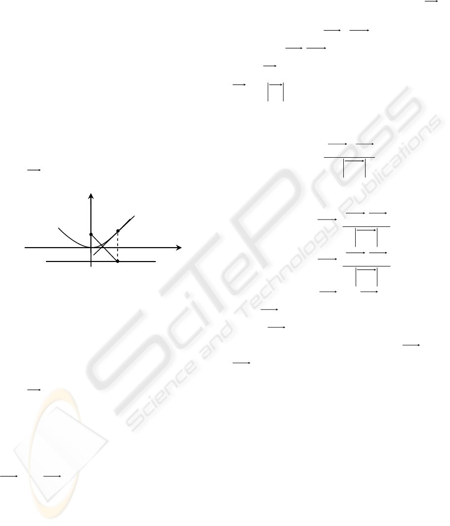
Geometric construction of a polygonal figure
skeleton is simple enough: it is a planar graph with
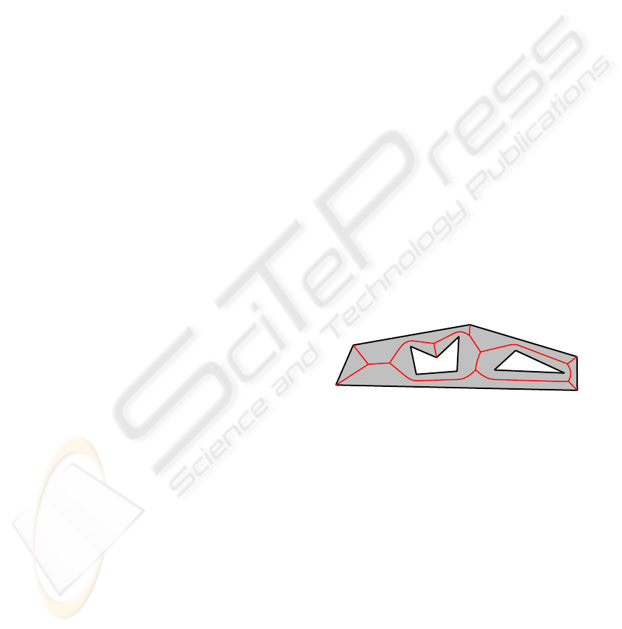
straight-line and parabolic edges (figure 1).
However, such analytical description of skele-
tons presents some difficulties. Presence of parabolic
edges gives rise to certain problems in constructing,
storing, processing, and utilizing skeletons in image
analysis. The general form for a parabola is
described by an implicit equation. This is not handy
for calculation of parabolas intersections, for
drawing and analysis.
Figure 1: A polygonal figure and its skeleton.
This shortcoming generates the tendency to
handle skeletons having no parabolic edges. This
idea is implemented in the concept of straight
skeleton (Aichholzer, Aurenhammer, 1996). But the
straight skeleton suffers from certain shortcomings,
videlicet: complexity of mathematical definition,
low algorithmic efficiency, regularization
complexity if noise effects are available.
In this paper, we propose a different method of
describing a skeleton in the form of a planar graph
with straight edges. To construct such a graph,
computing parabolic edges is not necessary either at
the step of the Voronoi diagram computing, or at the
steps of skeleton storing, drawing and processing,
respectively. This can be achieved as follows.
1. The skeleton of a polygonal figure is the union
of a set of the first and second order elementary
44
Mestetskiy L. (2010).
SKELETON REPRESENTATION BASED ON COMPOUND BEZIER CURVES.
In Proceedings of the International Conference on Computer Vision Theory and Applications, pages 44-51
DOI: 10.5220/0002831600440051
Copyright
c
SciTePress
Bezier curves. This union we call the compound
Bezier curve.
2. A compound Bezier curve is defined by its
control graph, which is obtained from the control
polygons of elementary Bezier curves. Every control
graph has linear edges.
Thus, to describe the skeleton, a straight-line
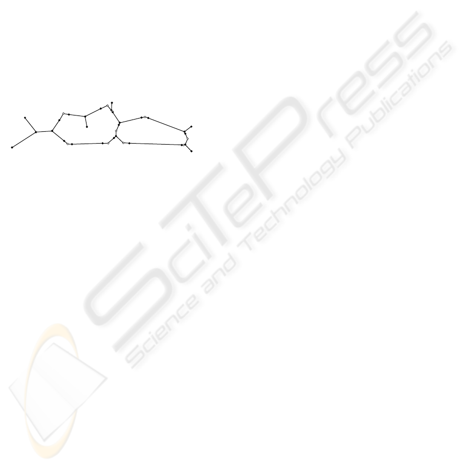
control graph is needed (figure 2).
The set of control graph vertices consists of two
subsets. The first subset is formed by vertices of
polygonal figure skeleton. And the second one
consists of the certain control points called handles
of Bezier curves.
2 STRUCTURE OF THE
SKELETON
Figure 2: The control graph of the skeleton from figure 1.
Terminal vertices are black and handle vertices are white.
Assume that
M
is a polygonal figure on
2
R with
the Euclidean distance
2
,),,( Rqpqpd ∈ . The
boundary of the figure
M
∂
consists of several
simple polygons.
An empty disk of the figure
M
of radius 0≥r
centered at a point
p is the closed point set
{
}
rqpdRqqpK
r
≤∈= ),(,:)(
2
such that
MpK
r
⊂)( .
A maximal empty disk (or, inscribed disk)
)(
max
pK
r
of the figure
M
is the empty disk that is
not contained in any other empty disks.
The skeleton
S of the figure
M
is the set of all
centers of maximal empty disks of the figure
{
}
∅≠∈= )(,:
max
pKMppS
r
.
This definition of the skeleton is more accurate
as comared to the one given in the introduction since
terminal vertices of skeletal graph are determined.
According to this definition all convex vertices of
the figure are terminal vertices of the skeleton. A
non-degenerate maximal empty disk touches the
figure boundary at least at two points. Every point of
the figure can be considered as a degenerate disk of
zero radius. These disks are empty ones because
they do not contain internal points and therefore, the
boundary points of the figure. Degenerate disks
centered at convex vertices of figure are maximal
empty disks because they are not contained in other
empty disks. Consequently, convex vertices of
polygonal figure are part of the skeleton.
A radial function is determined at every point of
skeleton. Radial function is equal to a radius of the
inscribed disk centered at this point. The radial
function assigns “the width” of figure relative to the
points of the skeleton.
Let
S be the skeleton of the polygonal figure
M
. The total number of points in the set S is
infinite, but it occurs that all these points are located
at the finite set of the straight-line and quadratic
parabolic segments. Let
Ss ∈ be a point of a
skeleton and
Mgg
∂
∈
21
, be the two closest
boundary points of
Ss
∈
. The points
1
g and
2
g
may have different positions on the figure boundary.
We shall name the boundary point by a corner point
if it is the vertex of polygonal figure, and simple
point otherwise. Three cases of
1
g and
2
g type
combinations are possible:
1
g and
2
g make a pair
of corner points, a pair of simple points or a corner
and a simple point.
If both
1
g ,
2
g are corner points then the point
Ss
∈
lies on the medial perpendicular of the
straight line segment
[
]
21
, gg (figure 3a).
If both points
1
g ,
2
g are simple and lie on
different sides of the figure then
s
is equidistant
from these sides. Then the point
s
lies on the
bisector of the angle, formed by these sides (figure
3b). If these sides are parallel then
s lies on the
straight line equidistant from these sides (figure 3c).
But if one of the points (for example,
1
g ) is
corner and the other (
2
g ) is simple then
s
is
equidistant from
1
g and from the side of polygon,
which contains
2
g . In this case
s
lies on the
parabola having a focus
1
g . And the directrix of
parabola is the side of polygon such that
2
g lies on
this side (figure 3d).
Thus, we distinguish three types of lines. The
first line (straight line) is defined by the pair “vertex-
vertex”, the second one (bisector) is defined by the
pair “side-side” and the third one (parabola) is
defined by the pair “vertex-side”. Every point of the
skeleton lies on one of these lines.
Let us use the following terminology. Vertices
and sides of polygonal figure are called sites. The
maximal connected subset of the skeleton
equidistant from the pair of sites is called middle
axis or, bisector. There are vv-bisectors, ss-bisectors
SKELETON REPRESENTATION BASED ON COMPOUND BEZIER CURVES
45
and vs-bisectors for the pairs of sites “vertex-
vertex”, “side-side” and “vertex-side”, respectively.
(c)
(a) (b)
(d)
s
g
1
g
2
s
g
1
g
2
g
1
s
g
2
s
g
1
g
2
Figure 3: Bisector types of polygonal figure.
3 SKELETON VERTICES
We aim to propose a method describing the skeletal
graph such that calculation of the equations of
parabolic bisectors is not needed.
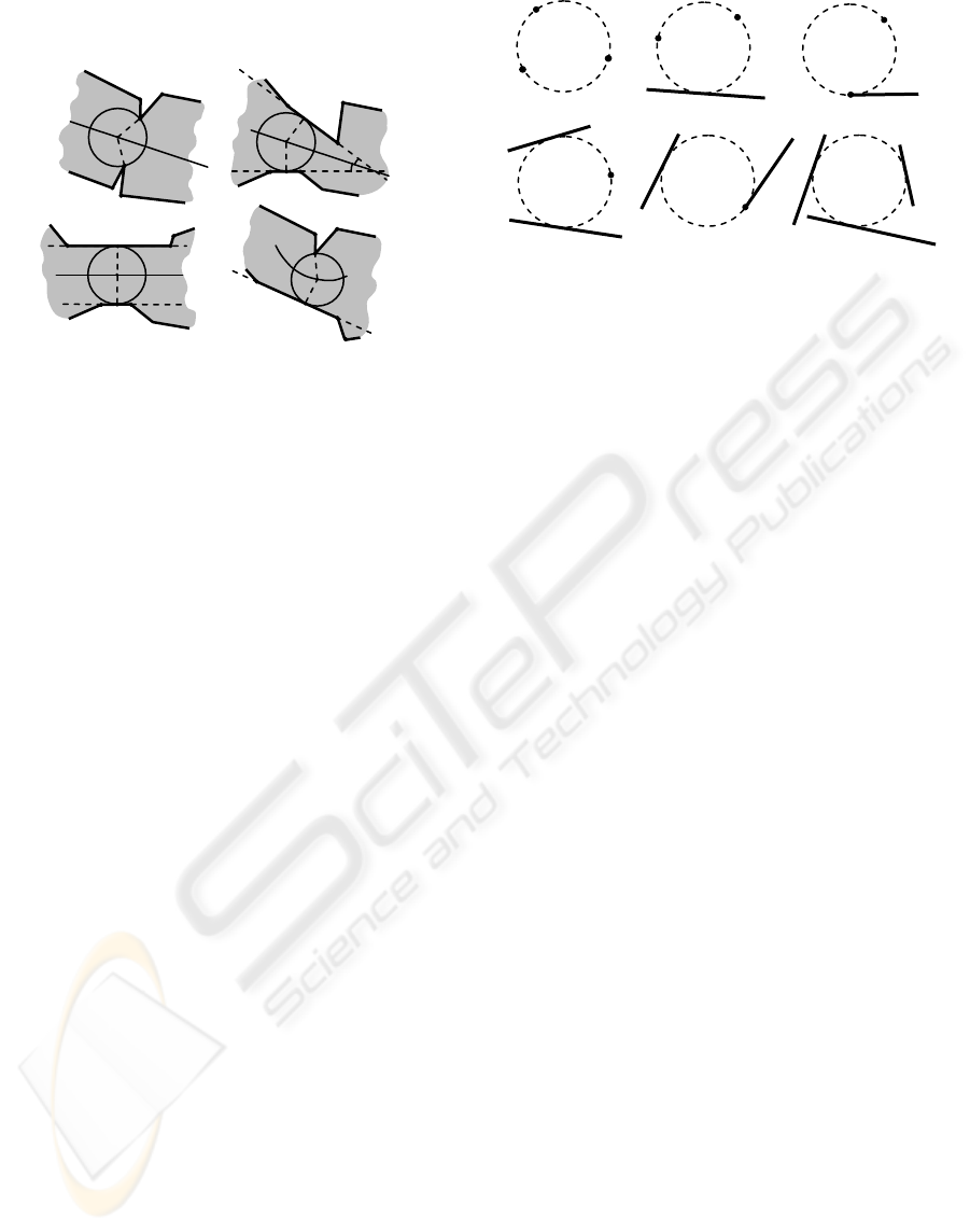
The skeleton vertices are equidistant to three or
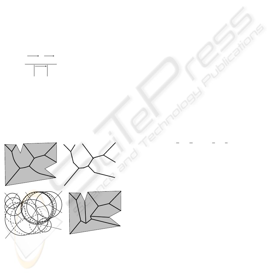
more sites. To find these vertices tangent circles can
be constructed for the triplets of sites. Calculation of
such circles involves a number of geometric tasks
(figure 4) related to the following combinations:
1) three vertex-sites (figure 4a);
2) two vertex-sited and one segment-site (figure
4 b,c);
3) two segment-sites and one vertex-site (figure
4 d,e);
4) three segment-sites (figure 4 f).
The second and third combinations involve two
cases depending on whether the vertex-sites match
the terminal points of segments.
Assume that the tangent circle exists and the
sequence of tangent points is defined. Then the
tangent circle is unique. To compute the center
t of
the circle tangent three sites
321
,, sss , the following
system of equation is to be solved:
⎪
⎩
⎪
⎨
⎧
=
=
),(),(
),(),(
3
2
1
2
2
2
1
2
stdstd
stdstd
In the cases in figures 4a,c,e,f both equations are
linear. But in the cases in figures 4b,d one equation
is linear, and the other is quadratic. After expressing
the Y-coordinate of the point
t
through the X-
coordinate in the linear equation it become possible
to reduce the second equation to the usual quadratic
equation, which is easily solved.
(a)
(b)
(
c
)
(d)
(e)
(f)
Figure 4: Tangent circles for the triplets of sites.
The obtained solution has to satisfy two auxiliary
conditions, which are easily checked. The first
condition requires the projections of
t
onto the
segment-sites to lie on these segments themselves.
The second condition requires the tangent circle to
lie inside the figure. This means the center of
tangent circle is required to lie to the left of the
segment-site.
4 SKELETON EDGES AS BEZIER
CURVE
Explicit description of the parametric curve
)),(),(()( tytxtV
=
]1,0[
∈
t provides handy tools to
deal with parabolic edges of skeleton.
)(tV
determines the skeleton edge with the vertices
)0(V
and
)1(V .
The main idea of our solution is that every
parabolic edge of the skeleton can be represented by
a quadratic Bezier curve
)()()()(
2
22
2
11
2
00
tBVtBVtBVtV ++= , ]1,0[∈t ,
where
22
0
)1()( ttB −= , )1(2)(
2
1
tttB −= ,
22
2
)( ttB = are
Bernstein polynomials. This curve is determined by
its control triangle
},,{
210
VVV . The points
0
V and
2
V are called the terminal points, and the point
1
V is
handle point of the Bezier curve.
0
V and
2
V are
vertices of skeleton, bat
1
V is not a skeleton vertex.
Such a way of edge description is compact and
easy-to-use since the only point together with two
terminal ones defines every edge. Also skeleton
drawing and handling becomes very simple since
various effective algorithms to handle Bezier curves
are known.
Generalized description is based on
representation of linear edges of the skeleton in the
VISAPP 2010 - International Conference on Computer Vision Theory and Applications
46
form of first order Bezier curves
)()()(
1
11
1
00
tBVtBVtV += , ]1,0[∈t .
Here points
0
V ,
1
V denote terminal points of
bisector.
ttB −=1)(
1
0
and
tVtB ⋅=
1
1
1
)(
are Bernstein
polynomials.
A parabolic skeleton edge is a vs-bisector. Let
A
and
B
be a pair of sites that assign this bisector.
Moreover, let
A
be a vertex and B be a side of
polygonal figure connecting vertices
1
B and
2
B .
We shall denote the side
B itself as well as a line
containing it by
21
BB . Without loss of generality, let
us assume the polygonal figure be left to the side
21
BB . Let us drop the perpendicular from the point
A
to the straight line
21
BB calling the intersection
D . Denote the middle of
A
D by O . The sites
A
and
B designate a rectangular Cartesian coordinate
system originated at
O and having DA as its Y-axis
and a line parallel to
21
BB as its X-axis (figure 5).
Given the sites
A
and B , the bisector of
A
and B consists of the centers of the circles touched
both
21
BB and
A
. Let
0
V and
2
V be the terminal
points of this bisector. And let
0
С and
2
С be the
projections of
0
V and
2
V onto the straight line
21
BB (figure 5).
Let us examine a point
),( yxV =
on the bisector
and its orthogonal projection
U on the straight line
21
BB . The point
A
coordinate pair is ),0( p . Since
22
UVAV = we obtain
222
)()( pypyx +=−+ .
Then the bisector parabolic equation is
2
4
1
x
p
y =
.
Given the points
),(
000
yxV = and ),(
222
yxV = ,
consider two lines tangent parabola at
0
V and
2
V .
x
y
O
A
D
C
0
С
2
V
0
V
2
V
U
B
1
B
2
Figure 5: Parabolic curve for vs-bisector.
As is known, the equation of a tangent line for a
curve
0),( =yxF at point )
ˆ
,
ˆ
( yx is
0)
ˆ
()
ˆ
,
ˆ
()
ˆ
()
ˆ
,
ˆ
( =−
⋅
′
+
−
⋅
′
yyyxFxxyxF
yx
.
In our case, we have
pyxyxF 4),(
2
−= . Then
the equations for tangent lines at the points
0
V and
2
V on the curve are the following:
0)(4)(2
000
=−
⋅
−
−
⋅
yypxxx
(1)
0)(4)(2
222
=−
⋅
−
−
⋅
yypxxx
(2)
Since
2
00
4
1
x
p
y =
,
2
22
4
1
x
p
y =
(3)
the solution of the system (1)-(2) is
)(
2
1
201
xxx += ,
(4)
201
4
1
xx
p
y =
(5)
Thus, we have obtained the point of tangent lines
intersection
),(
111
yxV
=
.
Permutation of Bernstein polynomials to the
quadratic Bezier curve equation gives the parametric
equations for Bezier curve
)(tV :
010
2
210
)(2)2()( xtxxtxxxtx +−−+−= (6)
010
2
210
)(2)2()( ytyytyyyty +−−+−= (7
)
]1,0[
∈
t .
Permutation of (4) to (6) presents
txxxtx ⋅
−
+
=
)()(
020
(8)
And permutation of (3) and (5) to (7) presents
[
]
=+−−+−=
2
020
2
0
22
220
2
0
)(2)2(
4
1
)( xtxxxtxxxx
p
ty
[
]
=+−−⋅−=
2
0200
22
20
)(2)(
4
1
xtxxxtxx
p
(9)
[]
2
020
)(
4
1
xtxx
p
−−=
From (8) and (9) we have
[]
2
)(
4
1
)( tx
p
ty =
, that
is the equation of the parabola of vs-bisector.
Thus, we have a parabolic bisector described as a
quadratic Bezier curve. This curve is assigned by a
control triangle
{
}
210
,, VVV . Two vertices
20
,VV are
terminal points of the bisector, and
1
V is the point of
intersection of tangents lines.
SKELETON REPRESENTATION BASED ON COMPOUND BEZIER CURVES
47
Consequently, in order to obtain bisector as the
Bezier curve it is necessary to calculate tangent lines
at the terminal points of bisector and to find their
intersection. Let us consider the solution of this
problem.
5 CONTROL TRIANGLE OF
SKELETON EDGE
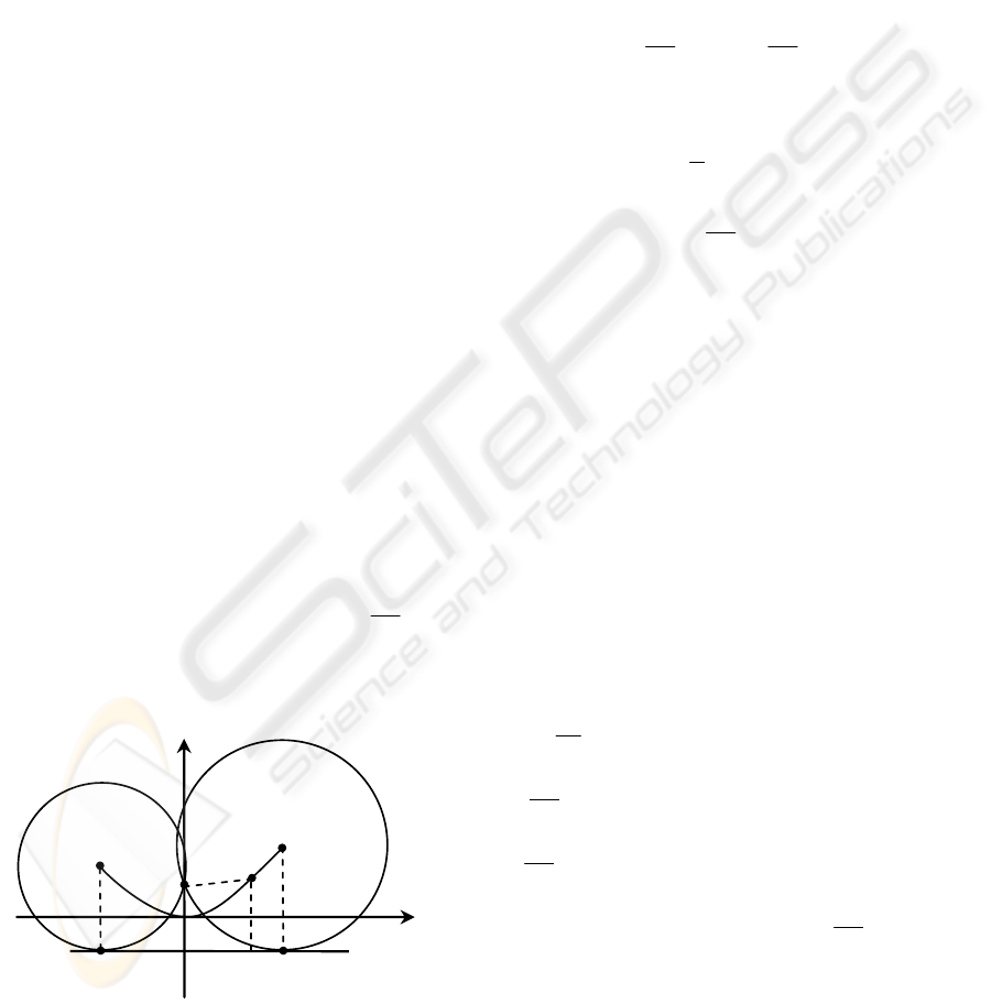
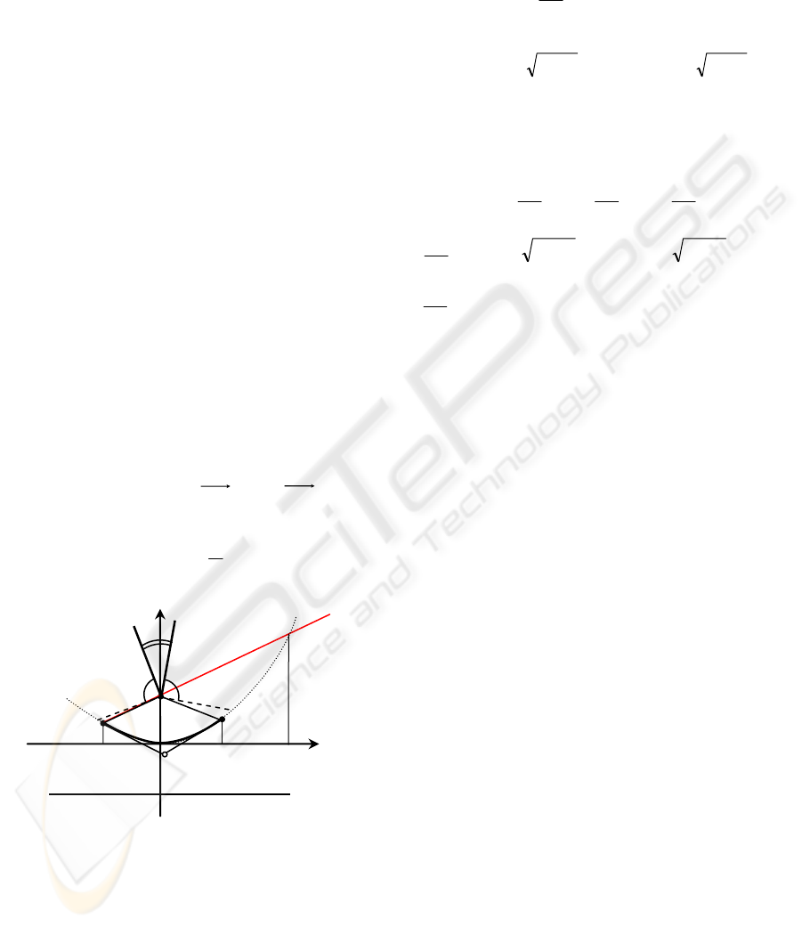
Let ),0( pA = be the focus of a parabola and
py −= be the directrix of the parabola. Assume that
the point
)
ˆ
,
ˆ
( yxV = lies on the parabola and
),
ˆ
( pxC −= is the projection of V onto the directrix
(figure 6). Let us show that a tangent line to a
parabola at the point
)
ˆ
,
ˆ
( yxV = is orthogonal to the
vector
AC .
x
y
p
С
V
A
‐
p
Figure 6: Orthogonality of tangent and direction from the
focus into the point of projection.
The equation of the tangent line to the parabola
04
2
=− pyx at the point )
ˆ
,
ˆ
( yxV = is
0)
ˆ
(4)
ˆ
(
ˆ
2 =
−
⋅−−⋅ yypxxx
(10)
We have that the vector
)4,
ˆ
2( px − is a normal
vector of the tangent line and is collinear to the
vector
AC .
This property makes it possible to find tangent
lines at the terminal points
0
V and
2
V of a skeleton
parabolic edge. This requires the projections
0
С and
2
С of
0
V and
2
V , respectively, onto the straight
line
21
BB to be calculated first. Then the vectors
0
AС and
2
AС are to be calculated. These vectors
are orthogonal to the corresponding tangent lines.
The source data to identify tangent lines to the
bisector at its terminal vertices is the following.
Given the pair of the sites
A
, B and two terminal
points
),(
000
yxV = , ),(
222
yxV = of bisector, let us
find the handle vertex
1
V of the control triangle
},,{
210
VVV . Without loss of generality, assume that
the site
A
is a vertex, the site B =[
1
B ,
2
B ] a side of
the polygonal figure and the polygonal figure lies to
the left of
B
.
Let us introduce the following notation. Let
PQ
denote the vector with an initial point
P
and a
terminal point
Q . By ][
2211
QPQP × denote the cross
product, by
(
)
2211
, QPQP denote the scalar product,
by
PQV + denote a shift of point V by vector
PQ , by PQ denote length of the vector.
The algorithm to solve the problem is following:
Algorithm steps
1. To find the parameter
p of the parabola:
21
121
2
][
BB
ABBB
p
⋅
×
=
.
2. To find points
0
С ,
2
С which are projections of
0
V ,
2
V , respectively:
(
)
21
0121
2110
,
BB
VBBB
BBBС
⋅+= ,
(
)
21
2121
2112
,
BB
VBBB
BBBС ⋅+=
.
3. To find vectors
0
AC and
2
AC :
),()..,..(
000
bayAyСxAxСAC =−−=
),()..,..(
222
dcyAyСxAxСAC =−−=
),( ba and ),( dc are coordinate pairs of
0
AC and
2
AC , respectively.
4. To solve the system of equations
⎩
⎨
⎧
=−⋅+−⋅
=−⋅+−⋅
0)()(
0)()(
22
00
yydxxc
yybxxa
5. The solution of the system gives the
coordinates of the handle point
),(
111
yxV = of the
control triangle.
6 SKELETAL GRAPH AS A
COMPOUND BEZIER CURVE
We showed that each parabolic edge of the skeleton
(vs-bisector) can be described by its quadratic Bezier
curve. For generality we can consider linear edges
(
vv-bisectors and ss-bisectors) to be linear Bezier
VISAPP 2010 - International Conference on Computer Vision Theory and Applications
48
curves
)()()(
1
11
1
00
tBVtBVtV +=
,
]1,0[∈t
. Here
points
0
V ,
1
V denote terminal points of bisector.
From
ttB −= 1)(
1
0
and tVtB ⋅=
1
1
1
)( we have
tVtVtV ⋅+−⋅=
10
)1()( .
Thus, the skeleton is a union of Bezier curves of
first- and second-order. We call this union the
“compound Bezier curve” analogously to the related
font design concept, where compound curves
describe the closed outlines of font symbols. In this
paper, curves describe more complex structure that
is a connected planar graph.
Planarity of the control graph of the compound
Bezier curve is an important property of the control
graph. This property can be proved as follows.
Let us examine the vertex-site
A
and the
segment-site B connected with the parabolic edge.
If points
0
V and
2
V lie on the same side of the
Y-axis, i.e.,
0
x and
2
x are of the same sign, then
from (5) it follows that
0
1
≥y and the point
1
V lies
above the segment
B
.
Assume that
0
x and
2
x have different signs
(figure 7). Since the focus
A
of the parabola is the
concave vertex of polygonal figure then the angle
α
, formed by incident sides of
A
, belongs to the
interval
π
α
π
2<< . Let us examine the angle
20
AVV∠ between vectors
0
AV and
2
AV . It is
obvious that
παπ
π
απ
<−=
⎟
⎠
⎞
⎜
⎝
⎛
⋅+−≤∠
2
22
20
AVV
x
y
A
V
0
V
2
x
0
α
B
V
*
x
2
x
*
π
/
2
π
/
2
V
1
Figure 7: Planarity of the control graph.
Consequently, the point
2
V lies below the
straight line
0
AV passing through the focus
A
, and
point
0
V . This straight line intersects parabola at the
point
0
V and at the point
∗
V with the coordinates
),(
∗∗
yx , moreover
2
xx >
∗
. The equation of the
straight line
0
AV is
x
apy ⋅+
=
, where a is the
angular coefficient. The points of intersection of this
straight line with the parabola can be found from the
equation
2
4
1
x
p
axp =+
.
This quadratic equation has two roots:
⎟
⎠
⎞
⎜
⎝
⎛
+−⋅= 12
2
0
aapx ,
⎟
⎠
⎞
⎜
⎝
⎛
++⋅=
∗
12
2
aapx .
Intersection point
1
V of the tangent lines has an
ordinate
1
y . From the equation (5) and the condition
2
xx >
∗
we obtain the following
estimation
==>=
∗
200201
4
1
4
1
4
1
xx
p
xx
p
xx
p
y
=
⎥
⎦
⎤
⎢
⎣
⎡
⎟
⎠
⎞
⎜
⎝
⎛
++⋅⋅
⎥
⎦
⎤
⎢
⎣
⎡
⎟
⎠
⎞
⎜
⎝
⎛
+−⋅= 1212
4
1
22
aapaap
p
[
]
paap
p
−=+−⋅= )1(4
4
1
222
.
We obtain
py
−
>
1
and the point
1
V lies above
the segment
B , too. Thus, we have that the control
triangle of a parabolic edge does not intersect its
own segment-site and lies inside the union of empty
circles centered at the points of a parabolic segment.
Consequently, the sides of a control triangle do not
have intersections with the remaining edges of
control graph. But this means that the control graph
of skeleton is planar.
7 RADIAL FUNCTION OF
SKELETON
To each point of a skeleton a radial function assigns
a radius to an inscribed empty disk centered at this
point. Let us examine representation of the radial
function if the skeleton is represented by the
compound Bezier curve.
Given the terminal points
0
V and
1
V of a linear
ss-bisector together with
0
r and
1
r , we can find the
radius of the empty disk centered at any inner point
of the edge
0
V
1
V (
0
r and
1
r are radii of the disks
centered at
0
V and
1
V , respectively). The radius of
empty disk centered at the point
tVtVtV
⋅
+
−
⋅
=
10
)1()( is
trtrtr ⋅
+
−
⋅
=
10
)1()(
(11)
Let us consider the vs-bisector case. In the local
coordinate system (figure 7) we have simple relation
between radii of disks and ordinates of the points of
SKELETON REPRESENTATION BASED ON COMPOUND BEZIER CURVES
49
bisector
ptytr += )()(
. From the property of
Bernstein polynomials
1)()()(
2
2
2
1
2
0
=++ tBtBtB we
obtain
=+++= ptBytBytBytr )()()()(
2
22
2
11
2
00
=⋅++⋅++⋅+= )()()()()()(
2
22
2
11
2
00
tBpytBpytBpy
)()()()(
2
22
2
11
2
00
tBrtBpytBr ⋅+⋅++⋅= .
Therefore
)()()()(
2
22
2
11
2
00
tBrtBrtBrtr ++= (12)
Let us consider the disc centered at the handle
point
1
V . For radius of this disk we have
pyr +=
11
. This disk is called a handle disk. As it
follows from geometric analysis (figure 7),
1
r is the
distance from the point
1
V to the line
21
BB . We
obtain:
21
1121
1
][
BB
VBBB
r
×
= .
Thus, the formulas (11) and (12) look like Bezier
splines.
Now let us consider the vv-bisector. All empty
disks centered at this bisector inner points touch the
common vertex of polygonal figure. Therefore the
radius of an empty disk centered at the point
tVtVtV ⋅+−⋅=
10
)1()( is defined as distance from
the point
)(tV to
A
.
(a
(b
(c)
(c)
Figure 8: Polygonal figure, its skeleton, control graph,
radial function, and straight skeleton.
We see that within the vv-bisector the raidus of
an empty disk can not be presented in Bezier spline
form. Thus, in order to compute the radial function
for any point of vv-bisector, coordintaes of related
concave vertices of polygonal figure should be
stored in the skeleton data structure. At the same
time, vs-bisector and ss-bisector require coordinates
of centers of handle disks as well as radii of handle
disks to be stored in the skeleton data structure.
The example in figure 8 shows the polygonal
figure and its skeleton (a), control graph of the
skeleton (b), and control disks of radial function (c).
Figure (d) shows the stright skeleton (Aichholzer,
Aurenhammer, 1996) for this polygon.
8 APPLICATIONS
Skeleton representation based on the compound
Bezier curve is a handy tool for visualization,
storage and image shape analysis in computer
vision.
To visualize the skeleton it is enough to utilize
standard graphic applications supporting drawing of
straight-line segments and Bezier curves as well.
Generally, graphic libraries are supplied with the
tools to draw cubic Bezier curves. To exploit such
programs in order to draw quadratic Bezier curves
the known conversion of control polygons is to be
carried out. A quadratic Bezier curve with the
control triangle
{
}
210
,, VVV matches the cubic Bezier
curve with the control quadrangle
{}
3210
,,, WWWW if
and only if
0
0
V
W
=
,
3
2
3
1
101
⋅+⋅= VVW
,
3
1
3
2
212
⋅+⋅= VVW
,
23
VW =
Thus, obtaining the control polygon of the cubic
Bezier curve matching the quadratic Bezier curve
can be represented.
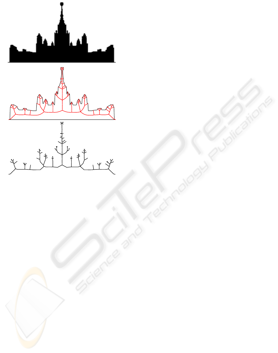
Example in the figure 9 presents an application
of our method to a natural image (binary bitmap
with the silhouette of Lomonosov Moscow
university).
Bezier representation of the polygonal figure
skeleton and family of its maximal empty disks
provide us with the opportunity to modify shape of
the figure. Modifying a figure shape based on
adjusting the skeleton and its radial function can be
used in computer graphics (Mestetskiy, 2000) and
image recognition to measure similarity of flexible
objects (Mestetskiy, 2007).
VISAPP 2010 - International Conference on Computer Vision Theory and Applications
50
(a
(b
(c)
Figure 9: Skeleton representation of natural image: (a)
binary bitmap, (b) polygonal figure approximation and the
skeleton, (c) the control graph of the skeleton.
9 CONCLUSIONS
In this paper, we have presented a new approach to
describe the skeleton of polygonal figure by stright
line control graph of compound Bezier curves. One
major advantage is the simplicity of this description.
Another advantage is the independence from the
algorithm of skeleton construction. The worst-case
running time for skeletal graph transformation to
compound Bezier curve is
)(nO
. Proposed form of
skeleton presents the tool for storing skeletons in
geographical databases and computer graphics
systems. We are currently working on extending the
above results to the segment Voronoi diagrams.
ACKNOWLEDGEMENTS
The author is grateful to the Russian Foundation of
Basic Researches, which has supported this work
(grants 08-01-00670, 08-07-00270).
REFERENCES
Aichholzer O., Aurenhammer F., 1996. Straight skeletons
for general polygonal figures in the plane. Lecture
Notes in Computer Science. Vol. 1090. Springer-
Verlag, 1996, 117-126.
Drysdale R., Lee D., 1978. Generalized Voronoi diagrams
in the plane. Proc. 16th Ann. Allerton Conf. Commun.
Control Comput., 1978, 833-842.
Fortune S., 1987. A sweepline algorithm for Voronoi
diagrams. Algorithmica, No. 2, 1987, 153-174.
Lee, D., 1982. Medial axis transformation of a planar
shape. IEEE Trans. Pat. Anal. Mach. Int. PAMI-4(4):
1982, 363-369.
Kirkpatrick D., 1979. Efficient computation of continuous
skeletons. Proc. 20th Ann. IEEE Symp. Foundations of
Computer Science, 1979, 18-27.
Mestetskiy, L., 2000. Fat curves and representation of
planar figures. Computers & Graphics, vol.24, No. 1,
2000, 9-21.
Mestetskiy L., Semenov A., 2008. Binary image skeleton -
continuous approach. In VISAPP’2008, Int. conf. on
computer vision theory and applications, INSTICC
Press, vol. 1, 2008, 251-258.
Mestetskiy L., 2007. Shape comparison of flexible objects
– similarity of palm silhouettes. In VISAPP’2007, 2
nd
Int. conf. on computer vision theory and applications,
INSTICC Press, vol. IFP/IA, 390-393.
Pfaltz, J. and Rosenfeld, A., 1967. Computer
representation of planar regions by their skeletons.
Communications of the ACM. , vol. 10, No. 2, 1967,
119 – 122.
Yap, C., 1987. An O(n log n) algorithm for the Voronoi
diagram of the set of simple curve segments. Discrete
Comput. Geom., No. 2, 1987, 365-393.
SKELETON REPRESENTATION BASED ON COMPOUND BEZIER CURVES
51
