
DETECTION OF ROAD CRACKS WITH MULTIPLE IMAGES
Sylvie Chambon
Laboratoire Central des Ponts et Chaussées, LCPC, Nantes, France
Keywords:
Default detection, Road, Crack, Matching, Stereovision, Fusion.
Abstract:
Extracting the defects of the road pavement in images is difficult and, most of the time, one image is used
alone. The difficulties of this task are: illumination changes, objects on the road, artefacts due to the dynamic
acquisition. In this work, we try to solve some of these problems by using acquisitions from different points
of view. In consequence, we present a new methodology based on these steps : the detection of defects in
each image, the matching of the images and the merging of the different extractions. We show the increase in
performances and more particularly how the false detections are reduced.
1 INTRODUCTION
In many countries, efforts are spent to reduce errors
and increase performances of the automatic (or semi-
automatic) evaluation of the quality of the road. This
quality depends on numerous characteristics: adher-
ence, texture and defects which include the snatching
parts, the repairs and the cracks. We focus on the de-
tection of cracks. Forty years ago, this evaluation was
manual: it is expensive, hard, dangerous for the em-
ployes, not reproducible and not efficient. Nowadays,
the detection of defects is made manually on acquisi-
tion of the road images (semi-automatic detection). It
is less dangerous than forty years ago, but, it is still
expensive, not efficient and not reproducible. In the
field of automatic analysis of cracks of the road sur-
face, different kinds of methods have been proposed
in the literature and even if they become more and
more efficient, we can notice two drawbacks that need
to be overcome: the detection presents a lot of false
detections and false negatives and they are are ded-
icated only to the detection of road cracks and they
are not able to detect other kind of defects. Conse-
quently, the aim of this work is to present a methodol-
ogy in order to reduce the number of false detections
with fusion of multiple detections on different images
of the same piece of road. In the first part of this pa-
per, we introduce a state of the art of detection of road
cracks. Then, we describe our methodology by giving
details about the acquisition, how the cracks are de-
tected, how the images are matched and finally how
all the results are used to give the final answer. The
last part shows the results in each step of the method-
ology before giving conclusions and perspectives.
2 ROAD CRACK DETECTION
In the context of detection with one image, four cat-
egories of techniques are identified. The Threshold
methods are the oldest ones and also the most popu-
lar (Acosta et al., 1992). These methods are simple
but the results contain a lot of false detections. The
methods by morphology (tools of mathematical mor-
phology), based on a previous thresholding (Tanaka
and Uematsu, 1998), allow to reduce false detec-
tions but strongly depend on the set of parameters.
The neuron networks-based methods have been pro-
posed to alleviate the problems of the two first cate-
gories (Kaseko and Ritchie, 1993). However, these
methods need a learning phase which is not well ap-
propriate to our task. The filtering methods are the
most recent and most of them are based on a wavelet
decomposition (Subirats et al., 2006) or on partial dif-
ferential equations (Augereau et al., 2001). We can
also notice an auto-correlation method (Lee and Os-
hima, 1994) and some methods also use the decom-
position of texture (Petrou et al., 1996). In the field
of the detection of road cracks with multiple images,
a method exploits a stereoscopic acquisition of the
scene (Wang and Gong, 2002) and the great advan-
tage is the complementarity of the different acquisi-
349
Chambon S. (2010).
DETECTION OF ROAD CRACKS WITH MULTIPLE IMAGES.
In Proceedings of the International Conference on Computer Vision Theory and Applications, pages 349-354
DOI: 10.5220/0002832903490354
Copyright
c
SciTePress
tions that helps to validate the detection. We have also
noticed that for the estimation of surface deformation,
stereo-correlation algorithms have been widely inves-
tigated (Sutton et al., 2008). It seems that even small
deformations can be characterized by such a system.
To resume, the mono-detection has shown its limit
(a high percentage of false detections) whereas the
multiple detections reveal great advantages (valida-
tion, possibility of detecting 3D defects) and are very
adapted to our task. Consequently, it seems natural to
investigate stereoscopic systems to detect cracks.
3 PROPOSED METHODOLOGY
The four steps of our methodology are:
(1) Acquisition of multiple images ;
(2) Crack detection in each image ;
(3) Matching of the images, i.e. to find the homolo-
gous pixels in the images ;
(4) Fusion of the results, i.e. to merge the different
detections by using the matching results.
Angle (0-20
◦
)
D = camera distance
C = distance camera-road
Piece of road
Ambiant light
Oriented light
Left camera Right camera
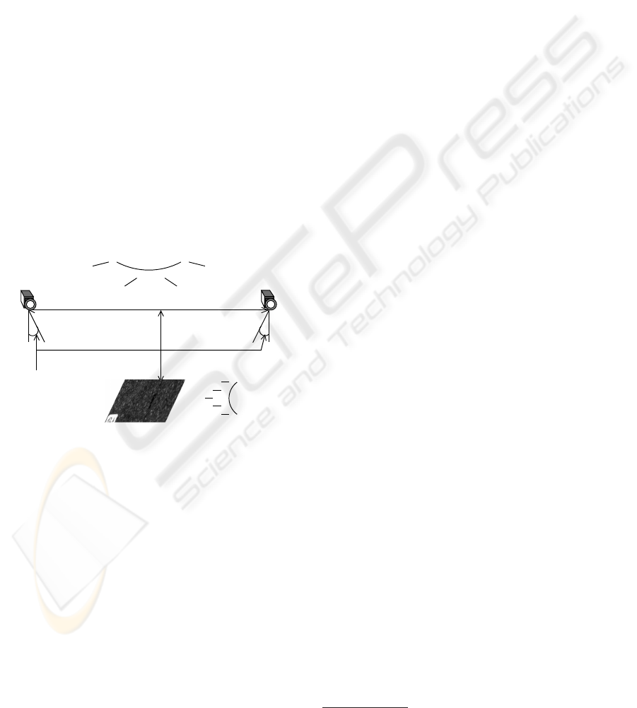
Figure 1: Acquisition system – It is composed of two cam-
eras. The angle of the cameras, the distances between the
two sensors, between the sensor and the scene, and the po-
sition of the lights are variable. The angle varies from 0 to
20
◦
and the distances between the cameras and between the
camera and the scene are adjusted to have good covering
between the two images. For the illumination, two options
are possible: ambient light or oriented light.
Acquisition. The quality of the detection results
strongly depends on the quality of the acquisition, see
Figure 2. Consequently, the choice of the acquisition
system is really important for the application and, this
is why in the literature, many systems have been pro-
posed and tested. A system is highly dependent on:
• The Type of the Sensor – Three types of sensors
can be distinguished: 2D sensors (that need image
processing technique), 3D sensors
1
(that are inde-
pendent from the lighting system) and the merg-
ing of 2D sensors and 3D sensors (Fukuhara et al.,
1990). We focus on 2D acquisition with cameras.
• The Number of Sensors – Most of the applications
use only one sensor or a mosaic of sensors (with
no covering between the different acquisitions).
(Wang and Gong, 2002) shows that using multi-
ple sensors can improve the performances and, in
this paper, we use two cameras.
• The Orientation of the Sensor – It influences the
quality of the results. In most of the proposed sys-
tems, the camera axis is perpendicular to the road
surface and we have tested different orientations:
a perpendicular position and an angular position
(with 10
◦
and 20
◦
), see Figure 1.
• The Consideration of the Illumination Changes –
They are one of the main difficulties. For solving
it, two possibilities are given: using natural light
or controlled light. Without controlled light, it is
necessary to pre-process the images for reducing
shadows and under/over-lighting areas, whereas,
with controlled light, these problems are less in-
fluent. However, the lighting system must be de-
signed in order to preserve the crack signal that
represents less than 1.5% of the images and is not
well contrasted with the road surface (Schmidt,
2003). An other way to solve illumination prob-
lem can be by using a stereoscopic system, how-
ever, in this work, we added a controlled illumina-
tion system in order to study both the contribution
of a stereoscopic system and the influence of the
type of light (Ambient light or Oriented light), see
Figure 1.
Crack Detection. We use a wavelet decomposition
analysis (Chambon et al., 2010) based on two steps:
first, to binarize images with a matched filtering and,
second, to refine the results with a Markov model-
based segmentation, see (Chambon et al., 2010) for
more details about the method and Figure 3 for an
example. Four variants are tested and compared in
this paper: Init, the initial work proposed in (Subirats
et al., 2006), Gaus, a variant that represents the crack
by a Gaussian function, InMM, the initial version with
an improvement of the Markov model-based segmen-
tation (new definition of the sites and of the poten-
tial function) and GaMM, Gaus with the new Markov
model, see Figure 3.
1
see http://phnx-sci.com/index.html
VISAPP 2010 - International Conference on Computer Vision Theory and Applications
350
(a)
ANGLE
0
◦
10
◦
20
◦
Ambient
Oriented
(b)
FIRST
IMAGE
SECOND
IMAGE
FIRST
DETAILS
SECOND
DETAILS
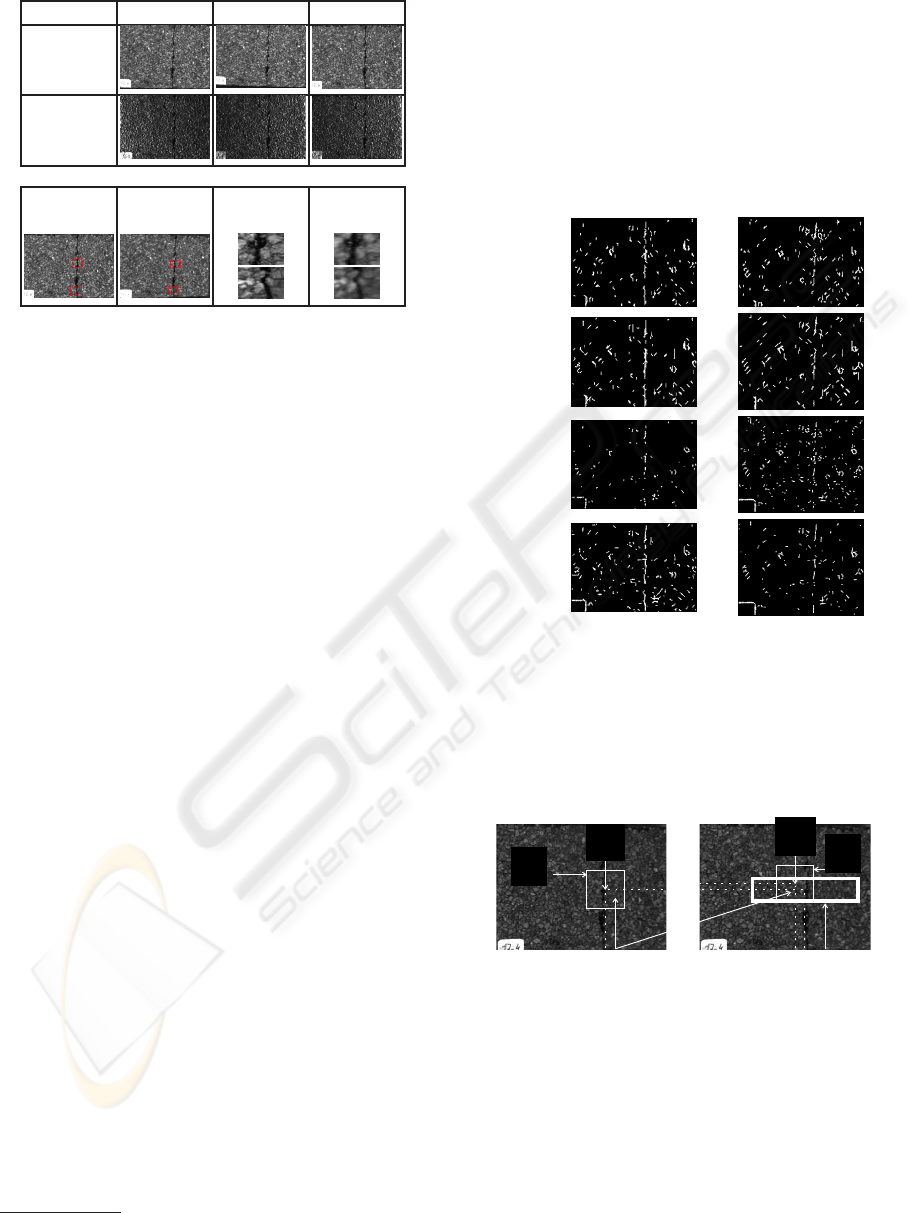
Figure 2: Acquisition conditions, see Figure 1 for the details
about the acquisition system – We can see the same piece
of road which is acquired with the 6 different possibilities
in (a). Visually, it seems that the crack is better contrasted
with Ambient illumination than with Oriented illumination.
The images in (b) give an illustration of the differences be-
tween two images of a stereoscopic pair. In the right part, it
represents the details of the red areas in the left part.
Matching. The goal of this step is to find correspon-
dent pixels in the two images, i.e. pixels that repre-
sent the same point of the scene. We consider p
1
i, j
the
pixel in the first image and p
2
k,l
its homologous pixel
in the second image. A lot of algorithms have been
proposed for stereoscopic matching. We can distin-
guish two kinds of methods: local ones, based on a
local similarity cost optimized with a winner take all
strategy, and global ones where a global cost on all the
correspondent pairs of pixels is optimized (Scharstein
and Szeliski, 2002). We work with high-textured im-
ages with no occlusion and it seems quite natural to
work with a local method. A correlation measure is
used and it evaluates how two sets of data are similar,
i.e. the grey levels of the two pixels and their neigh-
borhoods (which are contained in a correlation win-
dow). We have studied the advantages of correlation
measures and we decided to try five of them (the best
ones in our previous evaluation): the well known Nor-
malized Cross Correlation (NCC) which uses a scalar
product ; the Sum of Absolute Differences (SAD) ;
the Gradient Correlation (GC) based on the deriva-
tives of the images ; the RANK measure which evalu-
ates the dissimilarity between the rank of the data, i.e.
the grey levels in the correlation window (Zabih and
Woodfill, 1994) ; and finally, the Smooth Median Ab-
solute Deviation (SMAD) which evaluates the sum of
the h
2
first squared differences between the two cor-
relation windows. For more details on the correla-
2
Here, h is half of the size of the correlation window.
tion measures see (Chambon and Crouzil, 2003). The
matching algorithm is explained in Figure 4. More-
over, we add a symmetric constraint: matching is
done from the first image to the second and from the
second to the first and all correspondences that are
not coherent are removed, i.e. the pixels are consid-
ered as unmatched or undetermined. The results are
presented in section 4.
FIRST SECOND
Init
Gaus
InMM
GaMM
Figure 3: Crack detection – Examples of the results of the
four variants on one image, see image with 10
◦
and ambient
light in Figure 2. White pixels correspond to pixels consid-
ered as a crack. The Init and Gaus methods show a quite
dense detection, with a lot of false detections, whereas, the
two others are more sparse but with less false detections. A
quantitative analysis is given in section 4. For each variant,
it illustrates how the results are complementary.
M(f
1
i, j
, f
2
k,l
) ROI(p
1
i, j
)
f
1
i, j
p
1
i, j
p
2
k,l
f
2
k,l
Figure 4: Matching algorithm – For each pixel p
1
i, j
in the
first image, a region of interest, ROI(p
1
i, j
), is determined in
the second image. It corresponds to all the potential corre-
spondent pixels. For each pixel of ROI(p
1
i, j
), p
2
k,l
, a similar-
ity score or correlation score, M, is evaluated between the
grey levels of the pixels in their respective neighborhoods,
f
1
i, j
and f
2
k,l
, also called the correlation windows. The pixel
p
2
= argmax
k,l
M(f
1
i, j
, f
2
k,l
) (i.e. that obtains the best score)
is considered as the correspondent pixel of p
1
i, j
.
DETECTION OF ROAD CRACKS WITH MULTIPLE IMAGES
351

Table 1: Detection results – These values are the mean re-
sults obtained for the images with the best illumination con-
ditions, i.e. the ambient illumination.
METHOD IMAGE TP ACC FP FN DICE
Init First 10.41 22.81 66.78 16.30 0.51
Second 7.17 18.39 74.45 32.93 0.41
Gaus First 11.40 20.85 67.65 15.78 0.50
Second 7.14 17.72 75.14 32.21 0.40
InMM First 11.17 25.43 63.4 47.99 0.49
Second 5.93 18.04 76.02 37.26 0.41
GaMM First 8.86 21.05 70.09 12.81 0.49
Second 8.22 23.72 68.06 40.87 0.46
Fusion. We define the label function l that equals 0
when a pixelp is labelled as backgroundand 1 when it
is a crack. We also introduce the disparity function d
which equals the distance between a pixel and its cor-
respondent. This function equals −1 when no match
has been found. We propose an algorithm to merge
the results of matching and the two crack detections
based on two steps:
1. Initialization Step – Each pixel p
i, j
that ob-
tains the same label in the two views is validated
whereas the others are not, i.e.:
if ((l(p
1
i, j
) = l(p
2
k,l
)) & (d(p
1
i, j
) 6= −1))
then l(p
i, j
is validated.
else l(p
i, j
is considered as undetermined.
2. Iterative Step – The aims are to fill the undeter-
mined pixels and to add some points when there
are near pixels considered as crack. We use the
hypothesis that a crack is composed of a set of
connected segments with different orientations.
Consequently, we build a map of vote by estimat-
ing the cost of each path from the studied pixel
to the eight possible directions. More formally,
while the labels change:
For each validated pixels, we estimate a vote map
(local map), noted V, in a centered squared neigh-
borhood of size 2s+ 1
3
:
∀p
m,n
∈ V (p
i, j
), V(p
m,n
) =
s
∑
k=0
c(p
i+km, j+kn
) (1)
where V (p
i, j
) is the set of the 8 neighbors of p
i, j
and (m, n) corresponds to one of the 8 possible
directions and c is defined by:
c(p
i, j
) =
(
1 if l(p
i, j
) = 1
0 otherwise
(2)
3
In our experiments, the size of s equals the size of the
correlation window used for matching
We select p
d
defined by:
p
d
= argmax
p
m,n
(V(p
m,n
)), (3)
and finally:
l(p
d
) = 1
∀p ∈ V (p
i, j
)withp 6= p
d
, l(p
m,n
) = 0.
(4)
3. Final Step – At the end of the process, each un-
determined pixel is marked as background.
4 EXPERIMENTAL RESULTS
Evaluation Setup. We have tested 29 stereoscopic
acquisitions of the same piece of road. These images
have been manually segmented and we use this man-
ual segmentation as a reference for quantitative eval-
uation. For the detection, we evaluate the percentages
of: True Positives (TP), Accepted detections (ACC,
they correspond to pixels distant from 1 pixel from
the manual segmentation), False Positives (FP), False
negatives (FN). We also estimate the similarity coeffi-
cient, or DICE, which is equals to:
2TP
FN+P+FP
. In each
part of the analysis, we link the quality of the results
with the kind of acquisition.
Analysis of the Detection. It clearly appears that
for all the criteria, an Ambient light always permits to
obtain the best results, in particular, with an angle of
20
◦
. Table 1 shows the mean values of the criteria for
all the images with this illumination configuration. It
shows that results are different between the first view
and the second view and that the results in the both
views can be improved. A visual result is also pre-
sented in Figure 3.
Matching Results. We evaluate the quality of the
results with the density of the response (the percent-
age of pixelsthat are matched) and the execution time,
with different correlation window sizes, see Figure 5.
RANK obtains the best density and the best execution
time. With a window size lower than 9× 9, results are
quite bad and when the size is greater than 15 × 15
the density is not really improved(it highlights known
phenomenons). Visual results are presented with dis-
parity maps
4
, see Figure 6. The maps of RANK and
GC are the clearest ones, i.e. that present less false
negatives (black pixels). It also shows that SAD and
SMAD seem less sensitive to the difficulties in the
large black area on the bottom of the crack.
4
For each pixel, it gives the distance between the consid-
ered pixel and its correspondent: the clearer the pixel, the
larger the distance. Black pixels are unmatched pixels.
VISAPP 2010 - International Conference on Computer Vision Theory and Applications
352
EXECUTION TIME (in seconds for 9× 9 window)
NCC SAD GC RANK SMAD
121.1 156.7 1033.72 91.52 1410.38
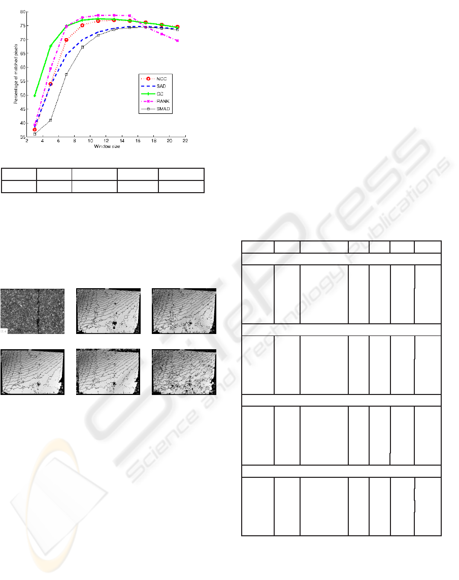
Figure 5: Density of matching and execution time – We
have estimated the disparities between the two images
with different sizes of correlation window. It appears that
RANK, GC and NCC obtain good density. The maximum
is reached between 9× 9 and 11× 11. All the results given
are the mean of the results obtained with the 29 couples.
First NCC SAD
GC RANK SMAD
Figure 6: Disparity maps – It shows typical results obtained
with this kind of images. Main problems are due to large
non-textured regions that correspond, in this case, to some
parts of the crack.
Fusion Results. The results of the fusion have been
quantitatively analyzed, see Table 2. The percentage
of good or accepted detections are higher than those
obtained with only one image whereas the percent-
age of false negatives is higher and consequently, the
DICE values are sometimes not better than the ini-
tial ones. The important aspect is that, as expected,
we have increased the reliability of the result but the
results are sparser. The percentage of TP+ACC is al-
ways improved, for each possible measure and each
possible detection method. The increase in perfor-
mances varies from 8 points to 22 points. In these
results, PD (Percentage Difference between the per-
centage of the correct detections in one image and the
percentage correct detections with the fusion of the
two detections) is always negative and means that the
fusion outperforms the initial results. In conclusion,
the reliability of the detection is higher whereas the
crack is less detected. The second analysis is that GC,
RANK and SMAD obtain better results than those
given by classic measures and it confirms that we need
a window size larger enough (more than 11 × 11) to
obtain reliable correspondences. Finally, it seems that
the Gaus method allows to obtain the most comple-
mentary results. An illustration of the results is given
in Figure 7. The detection maps given are clearer than
the ones given in Figure 3 but they are also sparser.
Table 2: Fusion results – For each measure (MEA.), we no-
tice the window size (WIN.) that permits to obtain the best
value of DICE. In brackets, we precise the differences be-
tween the percentage of TP+ACC obtained with each image
alone and with the fusion of the two results. The bold let-
ters indicate the best results for each criterion and the italic
letters illustrate when the DICE is better than using just one
image. PD is explained in § "Fusion result".
MEA. WIN. TP+ACC FP FN PD DICE
Init
NCC 19 45.6 (12.4) 54.4 70.1 -14.2 0.42
SAD 13 48.6 (15.4) 51.4 69.8 -13.2 0.43
GC 13 47 (13.7) 53 54.1 -6.3 0.54
RANK 15 47.2 (14) 52.8 52.1 -5.2 0.55
SMAD 19 49 (15.8) 51 53.2 -4.9 0.55
Gaus
NCC 9 54.3 (22) 45.7 70.8 -11.5 0.43
SAD 9 55.1 (22.8) 44.8 69.2 -10.3 0.45
GC 11 48.1 (15.7) 51.9 49.2 -2.9 0.57
RANK 15 48 (15.7) 52 52.5 -4.5 0.55
SMAD 19 49.4 (17.1) 50.6 54.2 -4.7 0.54
InMM
NCC 7 50.7 (14) 49.4 75.6 -6.7 0.38
SAD 11 52 (15.2) 48 73.3 -5.2 0.4
GC 21 41.5 (4.8) 58.5 67.2 -5.5 0.44
RANK 21 43.5 (6.8) 56.5 66.4 -4.5 0.45
SMAD 13 43.4 (6.7) 56.6 65 -3.9 0.46
GaMM
NCC 9 50.2 (20.2) 49.9 70.1 -11.1 0.42
SAD 11 48.1 (18.1) 51.9 70.7 -12 0.42
GC 13 38.2 (8.3) 61.8 59.9 -10.8 0.47
RANK 15 39.1 (9.2) 60.9 58.6 -9.9 0.48
SMAD 13 42 (12) 58 60.4 -9.5 0.48
5 CONCLUSIONS
In the field of the detection of road cracks, we pro-
posed an original methodology based on a stereo-
scopic system. Our contributions concern the propo-
sition of the generic algorithm, the study of the in-
DETECTION OF ROAD CRACKS WITH MULTIPLE IMAGES
353
fluence of different illumination conditions, the intro-
duction of different kind of correlation measures for
the matching step and how all the results are merged.
The results are quite encouraging and they highlight
the best conditions: acquisition with ambient illumi-
nation, detection with the method that considers the
crack as a Gaussian function and matching with a cor-
relation measure based on the gradients of the image.
Even if we have a specific application, i.e. crack de-
tection, this method can be used to detect other types
of defects in other type of difficult objects (low con-
trasted defects in highly textured objects). This work
can be improved and future work will introduce a
more systematic study of the influence of the light
position using (Drbohlav and Chantler, 2005). The
matching step will be evaluated quantitatively and the
tested images will be completed (with natural images
and different kind of textures). Finally, the 3D re-
construction step will be added to complete the crack
detection and include other defect detection, like the
snatching of pieces of road.
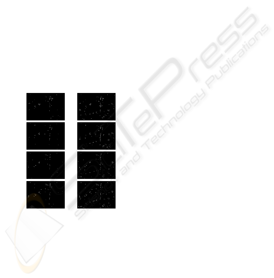
GC SMAD
Fusion
with
Init
Fusion
with
Gaus
Fusion
with
InMM
Fusion
with
GaMM
Figure 7: Detection maps with fusion method – Results are
shown for the same image as the results in Figure 3 and
only for two of the best correlation measures and for each
detection methods studied. It illustrates that the best perfor-
mances are reached with the Gaus detection method com-
bined with a GC matching.
REFERENCES
Acosta, J., Adolfo, L., and Mullen, R. (1992). Low-Cost
Video Image Processing System for Evaluating Pave-
ment Surface Distress. TRR: Journal of the Trans-
portation Research Board, 1348:63–72.
Augereau, B., Tremblais, B., Khoudeir, M., and Legeay, V.
(2001). A Differential Approach for Fissures Detec-
tion on Road Surface Images. In International Con-
ference on Quality Control by Artificial Vision.
Chambon, S. and Crouzil, A. (2003). Dense matching using
correlation: new measures that are robust near occlu-
sions. In BMVC.
Chambon, S., Gourraud, C., Moliard, J.-M., and Nicolle, P.
(2010). Road crack extraction with adapted filtering
and markov model-based segmentation. In VISAPP.
Drbohlav, O. and Chantler, M. (2005). On optimal light
configurations in photometric stereo. In ICCV, pages
1707–1712.
Fukuhara, T., Terada, K., Nagao, M., Kasahara, A., and
Ichihashi, S. (1990). Automatic pavement-distress-
survey system. ASCE, Journal of Transportation En-
gineering, 116(3):280–286.
Kaseko, M. and Ritchie, S. (1993). A neural network-based
methodology for pavement crack detection and clas-
sification. Transportation Research Part C: Emerging
Technologies information, 1(1):275–291.
Lee, H. and Oshima, H. (1994). New Crack-Imaging Proce-
dure Using Spatial Autocorrelation Function. ASCE,
Journal of Transportation Engineering, 120(2):206–
228.
Petrou, M., Kittler, J., and Song, K. (1996). Automatic sur-
face crack detection on textured materials. Journal of
Materials Processing Technology, 56(1–4):158–167.
Scharstein, D. and Szeliski, R. (2002). A Taxomomy and
Evaluation of Dense Two-Frame Stereo Correspon-
dence Algorithms. IJCV, 47(1):7–42.
Schmidt, B. (2003). Automated pavement cracking assess-
ment equipment – State of the art. Technical Report
320, Surface Characteristics Technical Committee of
the World Road Association (PIARC).
Subirats, P., Fabre, O., Dumoulin, J., Legeay, V., and Barba,
D. (2006). Automation of pavement surface crack de-
tection with a matched filtering to define the mother
wavelet function used. In EUSIPCO.
Sutton, M., Yan, J., Tiwari, V., Schreier, H., and Orteu, J.
(2008). The effect of out-of-plane motion on 2D and
3D digital image correlation measurements. Optics
and Lasers in Engineering, 46:746–757.
Tanaka, N. and Uematsu, K. (1998). A Crack Detection
Method in Road Surface Images Using Morphology.
In Workshop on Machine Vision Applications, pages
154–157.
Wang, K. and Gong, W. (2002). Automated Pavement Dis-
tress Survey: A Review and A New Direction. In
Pavement Evaluation Conference, pages 21–25.
Zabih, R. and Woodfill, J. (1994). Non-parametric Local
Transforms for Computing Visual Correspondence. In
ECCV, pages 151–158.
VISAPP 2010 - International Conference on Computer Vision Theory and Applications
354
