
GRAPH CUTS AND APPROXIMATION OF THE EUCLIDEAN
METRIC ON ANISOTROPIC GRIDS
Ondˇrej Danˇek and Pavel Matula
Centre for Biomedical Image Analysis, Faculty of Informatics, Masaryk University, Brno, Czech Republic
Keywords:
Graph cuts, Euclidean metric approximation, Anisotropic grids, Voronoi diagrams, Image segmentation.
Abstract:
Graph cuts can be used to find globally minimal contours and surfaces in 2D and 3D space, respectively.
To achieve this, weights of the edges in the graph are set so that the capacity of the cut approximates the
contour length or surface area under chosen metric. Formulas giving good approximation in the case of the
Euclidean metric are known, however, they assume isotropic resolution of the underlying grid of pixels or
voxels. Anisotropy has to be simulated using more general Riemannian metrics. In this paper we show how
to circumvent this and obtain a good approximation of the Euclidean metric on anisotropic grids directly by
exploiting the well-known Cauchy-Crofton formulas and Voronoi diagrams theory. Furthermore, we show
that our approach yields much smaller metrication errors and most interestingly, it is in particular situations
better even in the isotropic case due to its invariance to mirroring. Finally, we demonstrate an application of
the derived formulas to biomedical image segmentation.
1 INTRODUCTION
Graph cuts were originally developed as an elegant
tool for interactive image segmentation (Boykov and
Funka-Lea, 2006) with applicability to N-D problems
and allowing integration of various types of regional
or geometric constraints. Nevertheless, they quickly
emerged as a general technique to solve diverse com-
puter vision and image processing problems (Boykov
and Veksler, 2006). Particularly, graph cuts are suit-
able to find global minima of certain classes of en-
ergy functionals (Kolmogorov and Zabih, 2004) fre-
quently used in computer vision in polynomial time.
Among others, these may include energy terms de-
pendent on contour length or surface area. This is due
to (Boykov and Kolmogorov, 2003) who proved that
despite their discrete nature graph cuts can approxi-
mate any Euclidean or Riemannian metric with arbi-
trarily small error and derived the required formulas
for edge weights.
In the following text we focus on the Euclidean
metric as it is essential for graph cut based mini-
mization of many popular energy functionals such as
the Chan-Vese model for image segmentation (Chan
and Vese, 2001) (Zeng et al., 2006). The formu-
las derived in (Boykov and Kolmogorov, 2003) as-
sume isotropic resolution of the underlying grid of
pixels/voxels which is a limitation in some fields. For
instance, volumetric images produced by optical mi-
croscopes often have notably lower resolution in the
z axis than in the xy plane. Hence, before process-
ing it is necessary to either upsample the z direction
which substantially increases computational demands
or downsample the xy plane which causes loss of in-
formation. Last option is to simulate the anisotropy
using the more general Riemannian metrics. Unfor-
tunately, it turns out that the corresponding formu-
las have significantly larger approximation error that
once again can be reduced only for the price of slower
and more memory intensive computation taking into
account larger neighbourhood.
In this paper we show how to solve the above
mentioned problem and derive the weights required
for the approximation of the Euclidean metric on
anisotropic grids directly. For this purpose we fol-
low (Boykov and Kolmogorov, 2003) and exploit the
well-known Cauchy-Crofton formulas from integral
geometry. However, several amendments allow us to
obtain a better approximation. Namely, we employ
Voronoi diagrams theory to calculate the partitioning
of angular orientations of lines which is required dur-
ing the discretization of the Cauchy-Crofton formu-
las. This among other things makes our approxima-
tion invariant to image mirroring. Moreover,we show
that our approach has much smaller metrication error,
especially in the case of small neighbourhood or large
68
Dan
ˇ
ek O. and Matula P. (2010).
GRAPH CUTS AND APPROXIMATION OF THE EUCLIDEAN METRIC ON ANISOTROPIC GRIDS.
In Proceedings of the International Conference on Computer Vision Theory and Applications, pages 68-73
DOI: 10.5220/0002833000680073
Copyright
c
SciTePress
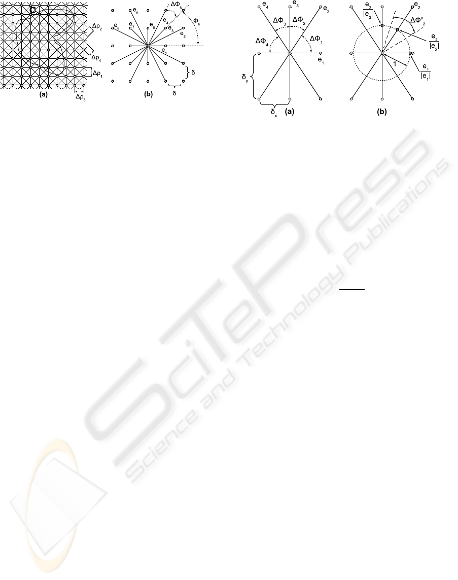
Figure 1: (a) 8-neighbourhood 2D grid graph. (b) 16-
neighbourhood system on a grid with isotropic resolution.
anisotropy and that under specific conditions it is bet-
ter even in the isotropic case.
The paper is structured as follows. The notation
and known results are briefly reviewed in Section 2.
In Section 3 we present our contribution and derive
the formulas approximating the Euclidean metric on
both 2D and 3D grids with anisotropic resolution.
Section 4 contains detailed discussion of the approxi-
mation error and gives example of an application of
our results to biomedical image segmentation. We
conclude the paper in Section 5.
2 CUT METRICS
Consider an undirected graph G embedded in a reg-
ular orthogonal 2D grid with all nodes having topo-
logically identical neighbourhood system and with
isotropic spacing δ between the nodes. Example of
such graph with 8-neighbourhood system is depicted
in Fig.1a. Further, let the neighbourhood system N
be described by a set of vectors N = {e
1
,...,e
n
}. We
assume that the vectors are listed in the increasing or-
der of their angular orientation 0 ≤ φ
k
< π. We also
assume that vectors e
k
are undirected (we do not dif-
ferentiate between e
k
and −e
k
) and shortest possible
in given direction, e.g. 16-neighbourhood would be
represented by a set of 8 vectors N
16
= {e
1
,...,e
8
}
as depicted in Fig.1b. Finally, we define the distance
between the nearest lines generated by vector e
k
in the
grid as ρ
k
(for 8-neighbourhood these are depicted in
Fig.1a).
Lets assume each edge e
k
is assigned particular
weight w
k
and imagine we are given a contour as
shown in Fig.1a. This contour divides the nodes of
the graph into two groups based on whether they lie
inside or outside the contour. A cut C is defined as the
set of all edges joining the inner nodes with the outer
ones. The cut capacity |C |
G
is the sum of the weights
of the cut edges. The question stands whether it is
possible to set weights w
k
so that the capacity of the
cut approximatesthe Euclidean length |C |
ε
of the con-
Figure 2: (a) 8-neighbourhood system on a grid with
anisotropic resolution. (b) Computation of ∆φ
v
2
.
tour. Since algorithms for finding minimal cuts con-
stitute well studied part of combinatorial optimiza-
tion (Boykov and Kolmogorov, 2004) this would al-
low us to effectively find globally minimal contours
or surfaces satisfying certain criterion.
The technical result of (Boykov and Kolmogorov,
2003) answers the question positively. Based on the
Cauchy-Crofton formula from integral geometry the
weights for a 2D grid should be set to:
w
k
=
δ
2
∆φ
k
2|e
k
|
(1)
The whole derivation of the formula is omitted here,
so is the extension to 3D grids. Both are being ex-
plained in more detail in the remaining text. Never-
theless, as already suggested in the introduction Eu-
clidean metric is not the only one that can be approxi-
mated using graph cuts. The complete discussion can
be found in (Kolmogorov and Boykov, 2005).
3 EUCLIDEAN METRIC ON
ANISOTROPIC GRIDS
Up until now we assumed that the grid of graph nodes
has isotropic resolution δ. In this section we investi-
gate the anisotropic case and adjust the edge weight
formulas appropriately.
3.1 2D Grids
Consider an undirected graph G embedded in a reg-
ular orthogonal 2D grid with all nodes having topo-
logically identical neighbourhood system. However,
let the spacing of the grid nodes be δ
x
and δ
y
in hori-
zontal and vertical directions, respectively. Otherwise
the whole notation remains unchanged. Example of
an 8-neighbourhood system over an anisotropic grid
is depicted in Fig. 2a.
GRAPH CUTS AND APPROXIMATION OF THE EUCLIDEAN METRIC ON ANISOTROPIC GRIDS
69
Now, consider the Cauchy-Crofton formula that
links Euclidean length |C |
ε
of contour C with a mea-
sure of a set of lines intersecting it:
|C |
ε
=
1
2
Z
n
c
dL (2)
where L is the space of all lines and n
c
(l) is the num-
ber of intersections of line l with contour C . Every
line in a plane is uniquely identified by its angular
orientation φ and distance ρ from the origin. Thus,
the formula can be rewritten in the form:
|C |
ε
=
Z
π
0
Z
+∞
−∞
n
c
(φ,ρ)
2
dρdφ (3)
and discretized by partitioning the space of all lines
according to the neighbourhood N = {e
1
,...,e
n
}:
|C |
ε
≈
n
∑
k=1
∑
i
n
c
(k,i)
2
∆ρ
k
!
∆φ
k
(4)
where i enumerates lines generated by vector e
k
. Fur-
ther, let n
c
(k) =
∑
i
n
c
(k,i) be the total number of in-
tersections of contour C with all lines generated by
vector e
k
. We obtain:
|C |
ε
≈
n
∑
k=1
n
c
(k)
∆ρ
k
∆φ
k
2
(5)
From the last equation it can be seen, that if we set
w
k
=
∆ρ
k
∆φ
k
2
(6)
then (proof omitted):
|C |
G
δ
x
,δ
y
→0
−−−−−−−−−−−−→
sup∆φ
k
→0,sup|e
k
|→0
|C |
ε
(7)
Finally, the distance between the closest lines gener-
ated by vector e
k
in the grid equals to:
∆ρ
k
=
δ
x
δ
y
|e
k
|
(8)
and if we substitute Eq.8 into Eq.6 we obtain the
above mentioned Eq.1.
So far we have followed the method of (Boykov
and Kolmogorov, 2003). However, when δ
x
6= δ
y
this
approach has a serious flaw. One may notice that in
the example depicted in Fig. 2a edges e
2
and e
4
will
be assigned different weights because ∆φ
2
6= ∆φ
4
and
∆ρ
2
= ∆ρ
4
. But this means that if we mirror the con-
tour horizontally we will obtain different cut capacity.
Hence, edge weights derived this way are not invari-
ant to mirroring, which is rather inconvenient prop-
erty causing additional bias of the approximation. In
fact, this bias is present in the isotropic case as well,
but not for all neighbourhoods. For instance, in the
16-neighbourhood depicted in Fig.1b edges e
2
and e
8
will be assigned different weights and it indeed has a
negative effect on the approximation as we will show
in the following section
The solution lies in different partitioning of the
unit circle of angular orientations. We do not uti-
lize ∆φ
k
in the way it has been used so far. Instead
we introduce new symbol ∆φ
v
k
which from a proba-
bilistic point of view can be interpreted as a measure
of lines closest to e
k
in terms of their angular ori-
entation. The computation is done as follows. Let
S = {
e
1
|e
1
|
,...,
e
n
|e
n
|
} be a set of points lying on a unit
circle. We calculate the Voronoi diagram of S on the
1D circle manifold and define ∆φ
v
k
to be the size of the
Voronoi cell corresponding to point
e
k
|e
k
|
. The whole
process is depicted in Fig. 2b. It reduces to the fol-
lowing formula:
∆φ
v
k
=
∆φ
k
+ ∆φ
k−1
2
(9)
Putting this together with Eq.6 and Eq.8 the final edge
weights for a 2D grid with anisotropic resolution are
calculated as:
w
′
k
=
∆ρ
k
∆φ
v
k
2
=
δ
x
δ
y
(∆φ
k
+ ∆φ
k−1
)
4|e
k
|
(10)
Such edge weights still follow the distribution of the
angular orientations of lines generated by vectors in
N but in a smarter way causing the approximation to
be invariant to contour mirroring while not breaking
the convergence of the original approach at the same
time.
3.2 3D Grids
In three dimensions the contour C is replaced by a
surface C
2
and the graph G is embedded in a reg-
ular orthogonal 3D grid with δ
x
, δ
y
and δ
z
spacing
between the nodes in x, y and z directions, respec-
tively, with all nodes having topologically identical
3D neighbourhood system N = {e
1
,...,e
n
} (e.g. 6-,
18- or 26-neighbourhood).
This time ∆ρ
k
expresses the ”density” of lines
generated by vector e
k
. It is calculated by intersect-
ing these lines with a plane perpendicular to them and
computing the area of cells in the obtained 2D grid of
points. It can be easily computed using this formula:
∆ρ
k
=
δ
x
δ
y
δ
z
|e
k
|
(11)
Each vector e
k
is now determined by two angular
orientations ϕ
k
and ψ
k
with ∆φ
k
corresponding to
the partitioning of the unit sphere among the angu-
lar orientations of vectors in N . In fact, this formu-
lation is rather vague and it is unclear how to cal-
culate ∆φ
k
the way it is being described in (Boykov
VISAPP 2010 - International Conference on Computer Vision Theory and Applications
70
0 2 4 6 8
−30
−20
−10
0
10
20
angular orientation
multiplicative error
Our
BK ’03
0 2 4 6 8
−6
−4
−2
0
2
4
angular orientation
multiplicative error
Our
BK ’03
0 2 4 6 8
−3
−2
−1
0
1
2
3
angular orientation
multiplicative error
Our
BK ’03
0 2 4 6 8
−3
−2
−1
0
1
2
angular orientation
multiplicative error
Our
BK ’03
0 2 4 6 8
−100
−50
0
50
100
150
angular orientation
multiplicative error
Our
BK ’03
0 2 4 6 8
−60
−40
−20
0
20
40
angular orientation
multiplicative error
Our
BK ’03
0 2 4 6 8
−25
−20
−15
−10
−5
0
5
10
angular orientation
multiplicative error
Our
BK ’03
0 2 4 6 8
−10
−5
0
5
10
angular orientation
multiplicative error
Our
BK ’03
0 2 4 6 8
−100
0
100
200
300
400
angular orientation
multiplicative error
Our
BK ’03
0 2 4 6 8
−100
−50
0
50
100
150
angular orientation
multiplicative error
Our
BK ’03
0 2 4 6 8
−60
−40
−20
0
20
40
60
angular orientation
multiplicative error
Our
BK ’03
0 2 4 6 8
−40
−30
−20
−10
0
10
20
30
angular orientation
multiplicative error
Our
BK ’03
N16
N8
N4
N32
1:1
3:1
6:1
Figure 3: Metrication error (in percents) in 2D for several combinations of neighbourhood system and anisotropy ratio.
and Kolmogorov, 2003). Particularly because for al-
most all common 3D neighbourhoods (e.g. 18- or 26-
neighbourhood) the distribution of the angular orien-
tations is not uniform (this stems from the fact, that
it is not possible to create a Platonic solid for such
number of points).
The capacity of a cut is analogously defined as the
sum of the weights of the edges joining grid nodes en-
closed by the surface C
2
with those lying outside and
the goal is to set the weights w
k
so that the capacity
of the cut approximates the area of the surface under
Euclidean metric. The Cauchy-Crofton formula for
surface area in 3D is:
|C
2
|
ε
=
1
π
Z
n
c
dL (12)
and using the same derivation steps as in the case of
2D grids yields the following edge weights:
w
k
=
∆ρ
k
∆φ
k
π
=
δ
x
δ
y
δ
z
∆φ
k
π|e
k
|
(13)
The problem with the clarity of ∆φ
k
is addressed
easily by extending our concept of Voronoi diagram
based weights ∆φ
v
k
. Let S = {
e
1
|e
1
|
,...,
e
n
|e
n
|
} be a set of
points this time lying on a unit sphere. We calculate
the Voronoi diagram of S on the 2D sphere surface
manifold and define ∆φ
v
k
to be the area of the Voronoi
cell corresponding to point
e
k
|e
k
|
. This is a general
and explicit approach that can be used for any type
of neighbourhood. Unfortunately, the spherical case
can not be reduced to a simple formula. To compute
the spherical Voronoi diagram we recommend to use
the convex hull based method described in (Brown,
1979). Putting this all together we end up with the
final formula for 3D anisotropic grids:
w
′
k
=
∆ρ
k
∆φ
v
k
π
=
δ
x
δ
y
δ
z
∆φ
v
k
π|e
k
|
(14)
To conclude this section, this approach can be the-
oretically extended to any number of dimensions. In
the general N-D case one would have to calculate
Voronoi diagram of points on a hypersphereto get ∆φ
v
k
weights. The adjustment of ∆ρ
k
is straightforward.
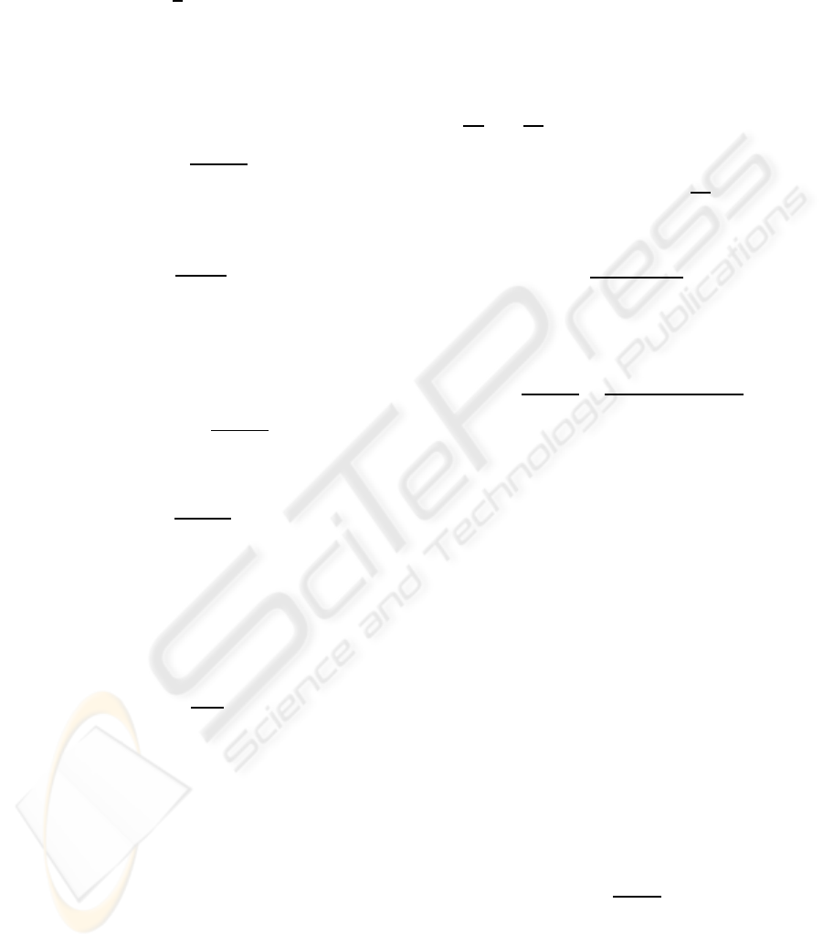
4 EXPERIMENTAL RESULTS
4.1 Approximation Error
To benchmark the approximations we chose to mea-
sure the multiplicative error they give under partic-
ular angular orientations in 2D. Graphs of the er-
ror are available in Fig. 3. The figure contains 12
graphs where each column corresponds to a partic-
ular 2D neighbourhood and each row to a particu-
lar anisotropy ratio. We compared our approxima-
tion with the method described in (Boykov and Kol-
mogorov,2003). To simulate the anisotropy we had to
embed it into a Riemannian metric in the latter case.
According to the referenced paper the weights for a
GRAPH CUTS AND APPROXIMATION OF THE EUCLIDEAN METRIC ON ANISOTROPIC GRIDS
71
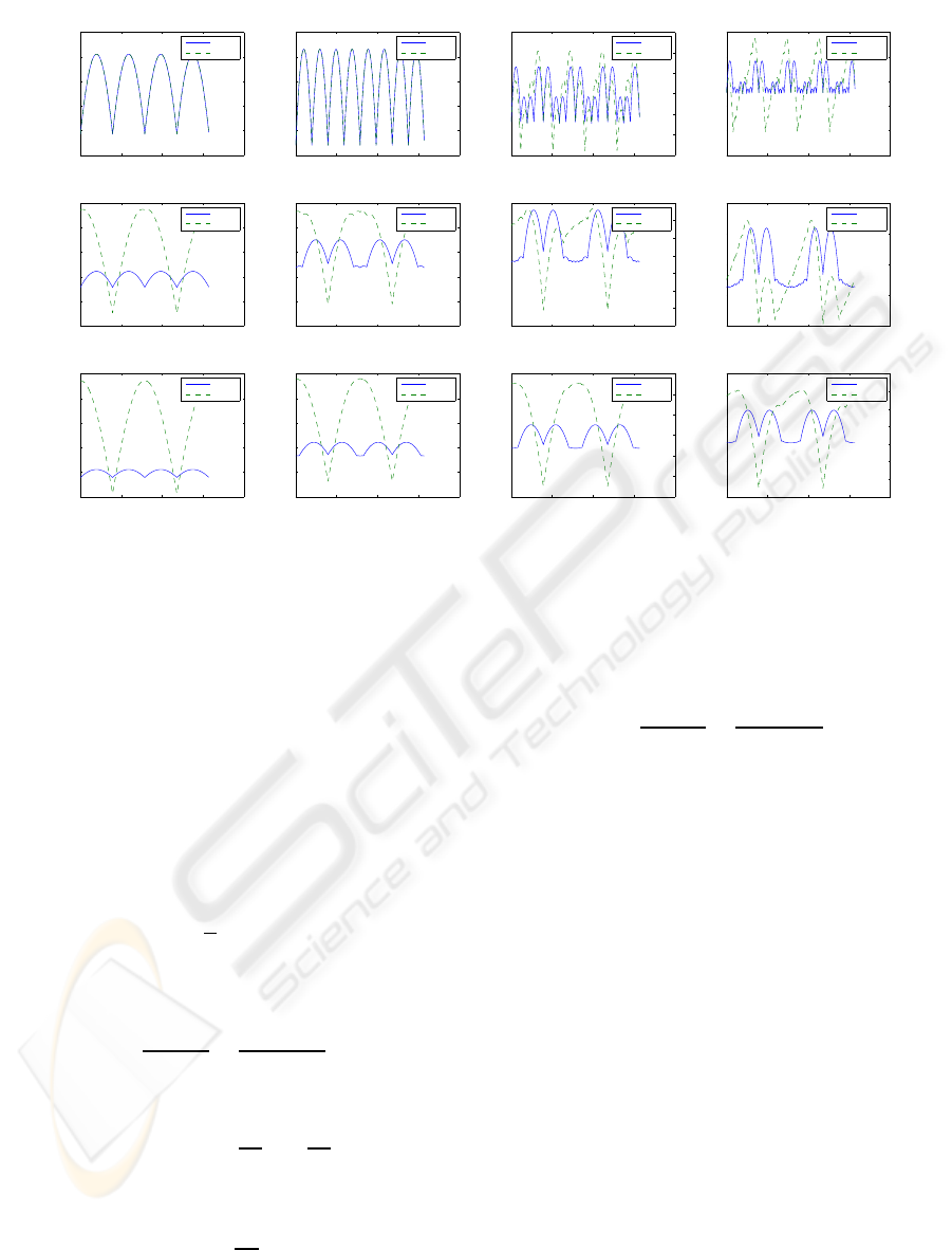
Figure 4: Two examples of biomedical image segmentation using the Chan-Vese model. (a) yz cross-section of the segmented
image. (b) Level-set based method. (c) Graph cuts with edge weights for isotropic resolution. (d) Graph cuts with anisotropy
embedded into the Riemannian metric. (e) Graph cuts with our edge weights.
Riemannian metric with a constant metric tensor D
over an isotropic 2D grid should be set to:
w
R
k
=
δ
2
∆φ
k
2|e
k
|
·
detD
(u
T
k
· D· u
k
)
3/2
(15)
where u
k
=
e
k
|e
k
|
and to:
w
R
k
=
δ
3
∆φ
k
π|e
k
|
·
detD
(u
T
k
· D· u
k
)
2
(16)
in case of a 3D grid. Resolution change corresponds
to a constant metric tensor with eigenvectors aligned
with the coordinate system and eigenvalues δ
2
x
and δ
2
y
.
Hence, the metric tensor simulating the anisotropic
grid has the following form:
D =
δ
2
x
0
0 δ
2
y
(17)
Notice that if D is the identity matrix the second term
in Eq.15 and Eq.16 vanishes and the formulas reduce
to the isotropic case.
The multiplicative error measures in percents the
difference between the approximated value and the
factual length, i.e. zero is the ideal meaning no er-
ror. As can be seen from Fig. 3 both approaches per-
form equivalently in the isotropic case for 4- and 8-
neighbourhood. For larger neighbourhoods our ap-
proach is almost two times better and its invariance
to mirroring is also apparent as the graph is sym-
metrical around values
π
2
, π and
3π
2
. With increasing
anisotropy the gap widens and especially for smaller
neighbourhoods the difference is really huge. How-
ever, note that the maximal error depends primarily
on sup ∆φ
k
and that this value increases with increas-
ing anisotropy. Thus, for high anisotropy ratios using
larger neighbourhood is inevitable.
4.2 Applications to Image Segmentation
In this subsection we show the practical impact of our
results and evaluate the benefits of the improved ap-
proximation in biomedical image segmentation. We
chose the Chan-Vese segmentation model (Chan and
Vese, 2001) that is being very popular in this field
for its robust segmentation of highly degraded data.
The Chan-Vese model is a binary segmentation model
VISAPP 2010 - International Conference on Computer Vision Theory and Applications
72

which corresponds to piecewise-constant specializa-
tion of the well-known Mumford-Shah energy func-
tional. In simple terms, it segments the image into
two regions trying to minimize the length of the fron-
tier between them and their intensity variance. This
functional can be minimized using graph cuts (Zeng
et al., 2006) and as it tries to minimize the boundary
length it obviously depends on the Euclidean metric
approximation.
To test the improvement of our approximation
over the previous approach also in 3D we plugged
the derived formulas into the algorithm and used it to
segment low-quality volumetric images of cell clus-
ters acquired by an optical microscope. The yz cross-
sections of the segmented images are depicted in
Fig.4a. The dimensions of the images are 280×360×
50, with resolution in the xy plane being about 4.5
times the resolution in the z direction. We used 26-
neighbourhood to segment the images.
In Fig. 4b is the Chan-Vese segmentation com-
puted using level-sets. This technique was much
slower than the graph cuts, however, it does not suf-
fer from the metrication errors so we used its results
as the ground truth. Figure 4c shows the graph cut
based segmentation when the anisotropy is ignored.
The results obtained using the Riemannian metric and
our weights are depicted in Fig. 4d and Fig. 4e, re-
spectively. Clearly, our method gives a result closest
to the level-sets. On the other hand, the segmenta-
tion based on the Riemannian metric seems too flat
or chopped. Based on the results from the previous
subsection it could be probably greatly improved us-
ing a larger neighbourhood, but at the cost of higher
computational demands.
5 CONCLUSIONS AND FUTURE
WORK
In this paper we addressed the problem of approxima-
tion of the Euclidean metric on 2D and 3D anisotropic
grids via graph cuts. We derived the required formu-
las and showed that our approach has a significantly
smaller metrication error than the previous one and
that it is invariant to image mirroring. Using the pre-
sented results it is possible to exploit graph cut based
energy minimization dependent on contour length or
surface area over images with anisotropic resolution
directly without the need to resample them or to use
large neighbourhoods for better precision. A possi-
ble application of the results was demonstrated on a
biomedical image segmentation.
As explained in Section 4.1 anisotropic grids cor-
respond to a special case of the Riemannian met-
ric with a constant metric tensor with eigenvectors
aligned with the coordinate system. However, the
general case of this metric is also being widely used
in several fields including image segmentation. Tak-
ing into account the relatively high error of the current
formulas we would like to make use of the presented
results and focus on better approximations of the gen-
eral case of the Riemannian metric in our future work.
ACKNOWLEDGEMENTS
This work has been supported by the Ministry of Ed-
ucation of the Czech Republic (Projects No. MSM-
0021622419, No. LC535 and No. 2B06052).
REFERENCES
Boykov, Y. and Funka-Lea, G. (2006). Graph cuts and effi-
cient n-d image segmentation (review). International
Journal of Computer Vision, 70(2):109–131.
Boykov, Y. and Kolmogorov, V. (2003). Computing geo-
desics and minimal surfaces via graph cuts. In ICCV
’03: Proceedings of the Ninth IEEE International
Conference on Computer Vision, page 26.
Boykov, Y. and Kolmogorov, V. (2004). An experi-
mental comparison of min-cut/max-flow algorithms
for energy minimization in vision. IEEE Transac-
tions on Pattern Analysis and Machine Intelligence,
26(9):1124–1137.
Boykov, Y. and Veksler, O. (2006). Graph cuts in vision and
graphics: Theories and applications. In Handbook of
Mathematical Models in Computer Vision, pages 79–
96. Springer-Verlag.
Brown, K. Q. (1979). Geometric transforms for fast geo-
metric algorithms. PhD thesis, Pittsburgh, PA, USA.
Chan, T. F. and Vese, L. A. (2001). Active contours with-
out edges. IEEE Transactions on Image Processing,
10(2):266–277.
Kolmogorov, V. and Boykov, Y. (2005). What metrics can
be approximated by geo-cuts, or global optimization
of length/area and flux. In ICCV ’05: Proceedings
of the Tenth IEEE International Conference on Com-
puter Vision, pages 564–571.
Kolmogorov, V. and Zabih, R. (2004). What energy func-
tions can be minimized via graph cuts? IEEE Trans-
actions on Pattern Analysis and Machine Intelligence,
26(2):147–159.
Zeng, Y., Chen, W., and Peng, Q. (2006). Efficiently solv-
ing the piecewise constant mumford-shah model using
graph cuts. Technical report, Dept. of Computer Sci-
ence, Zhejiang University, P.R. China.
GRAPH CUTS AND APPROXIMATION OF THE EUCLIDEAN METRIC ON ANISOTROPIC GRIDS
73
