
CONTROLLED AND ADAPTIVE MESH ZIPPERING
Stefano Marras
1
, Fabio Ganovelli
2
, Paolo Cignoni
2
, Riccardo Scateni
1
and Roberto Scopigno
2
1
University of Cagliari, Italy
2
ISTI-CNR, Italy
Keywords:
Zippering, Stitching, 3D scanning.
Abstract:
Merging meshes is a recurrent need in geometry modeling and it is a critical step in the 3D acquisition pipeline,
where it is used for building a single mesh from several range scans. A pioneering simple and effective
solution to merging is represented by the Zippering algorithm (Turk and Levoy, 1994), which consists of
simply stitching the meshes together along their borders. In this paper we propose a new extended version
of the zippering algorithm that enables the user to control the resulting mesh by introducing quality criteria
in the selection of redundant data, and allows to zip together meshes with different granularity by an ad hoc
refinement algorithm.
1 INTRODUCTION AND
PREVIOUS WORK
In recent years, the technology for digitizing real
3D objects has greatly improved and became more
accessible to the general audience. While only
ten years ago the acquisition of the Michelangelo’s
David (Pereira et al., 2000) required 22 people for 30
days and the prototypical device sampled 14k points
per second, nowadays it is possible to acquire a sim-
ilar device for less than 3000$ (NextEngine, 2010).
However, notwithstanding the impressive improve-
ment and diffusion of the hardware, the 3D scanning
software pipeline is substantially unchanged: once the
single range maps have been acquired with the device,
they must be aligned in the same reference system,
then merged in a single triangle mesh. After these
steps others may follow for including colors and/or
for optimizing the resulting mesh for rendering. ai
Over the years each and every step has been refined
in several regards, and nowadays we can safely state
that the 3D acquisition pipeline is a stable process.
Nonetheless, further improvements still can be done
for example in terms of computation time, which is
what we do in this work, focusing on the process of
merging aligned range maps.
A range map is an image where each pixel stores a
depth value, which means that information contained
in a range map is a set of points in 3D space. Given
the regular distribution of the samples in the image
space, it is possible to triangulate them to obtain a
triangle mesh for each range map.
An early mesh merging approach, called zipper-
ing (Turk and Levoy, 1994), consists in stitching to-
gether the pairs of triangulations that overlap in 3D
space by eliminating the redundant faces in the over-
lapping regions and then adjusting the mesh connec-
tivity locally. Other approaches work by triangu-
lating union of the point sets, like the Ball Pivot-
ing (Bernardini et al., 1999), which consists of rolling
an imaginary ball on the point sets and creating a tri-
angle for each triplet of points supporting the ball.
This approach is strictly connected to the idea of α-
shapes (Edelsbrunner and M
¨
ucke, 1994), which may
be thought as a ball pivoting where the ball may ap-
pear simultaneously everywhere outside the scanned
volume. In other approaches, like in (Duan and Qin,
2003), active contours are used to deform a mesh to
fit the sample points. Note that in these cases the ver-
tices of the final mesh do not coincide with the initial
samples. In fact, the reconstruction of the final repre-
sentation is also a way to filter the input data to reduce
noise and discard outliers.
Imperfections and noise produced by the scanning
devices is one of the reasons for the success of vol-
umetric methods, which convert the range maps in
a volumetric domain (a discrete distance field), well
suited for filtering and merging operations. The Space
Carving proposed in (Curless, 1999) uses range maps
and line of sight of the scanner to determine a con-
figuration of the empty voxels consistent with all the
range images. Many of the improvements to volu-
104
Marras S., Ganovelli F., Cignoni P., Scateni R. and Scopigno R. (2010).
CONTROLLED AND ADAPTIVE MESH ZIPPERING.
In Proceedings of the International Conference on Computer Graphics Theory and Applications, pages 104-109
DOI: 10.5220/0002834301040109
Copyright
c
SciTePress
metric methods consist of enhanced methods for es-
timating distances and normals of the surface. The
method proposed in (Hoppe et al., 1992) uses local
estimation of tangent planes to obtain a signed dis-
tance function. More recent approaches uses MLS
local approximations of the surface to address con-
tinuity of the distance function (Alexa et al., 2001;
Shen et al., 2005) which may be then visualized by
sampling the isosurface with points, using contour-
ing techniques (Fiorin et al., 2007) to build a poly-
gon mesh or ray tracing it at rendering time (Guen-
nebaud and Gross, 2007). A quadratic local approx-
imation scheme has been combined with a hierarchi-
cal space subdivision that allows the reconstructions
of the surface for large number of points in (Ohtake
et al., 2003). In the same flavor, the Poisson Surface
Reconstruction algorithm (Kazhdan et al., 2006) for-
mulates the problem of defining the surface from a set
of point as a Poisson problem, for which a least square
solution can be efficiently found at different scales.
The revisitation of the mesh zippering as a mesh
merging algorithm is mainly motivated by the fact
that, thanks to the improvement of both the soft-
ware and the hardware involved in the 3D scanning
pipeline, the quality of acquisition and range maps
alignment may allow to zip them together and to ob-
tain the same result as with more costly and sophisti-
cated methods.
2 ALGORITHM OVERVIEW
Our zippering algorithm consists of the same steps
as the original version presented in (Turk and Levoy,
1994), that we summarizes in the following. Given
two meshes A and B that partially overlap, the zipper-
ing algorithm proceeds in three phases:
• Border Erosion. Remove faces from the border
of the patches to minimize data redundancy.
• Clip a patch against the other. The border of
one of the two range maps is projected on the
other range map, the faces intersected by projec-
tion of A’s border are retriangulated in order to
create a new consistent connectivity.
• Cleaning. Improve the quality of the mesh in the
region when retriangulation occurred.
These phases are revisited to extend the zipper-
ing to support a user-defined criterion to eliminate the
data redundancy and to robustly support the zippering
of patches with very different resolution.
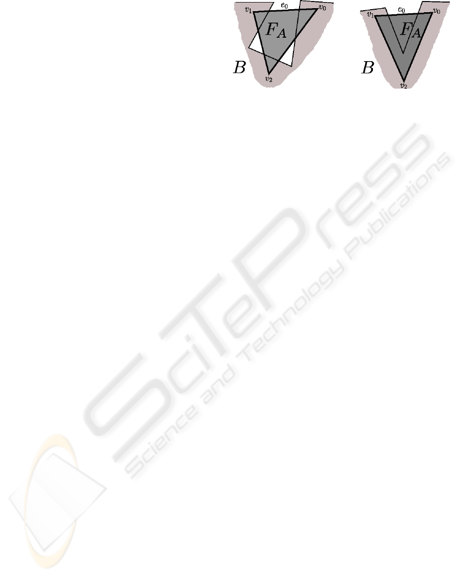
Figure 1: False Positive.
2.1 Border Erosion
In the original zippering algorithm (Turk and Levoy,
1994) a triangular face is said to be redundant if its 3
vertices project on the surface of the other patch. As
it is shown in Figure 1 this process may easily create
holes of roughly the size of the face, that will be even-
tually triangulated after the zippering process. How-
ever there are situations in which we cannot make the
assumption that range maps to be zippered are simi-
lar in terms of size and number of polygons, for ex-
ample because more than one device is used to scan
the surface and the two produce range maps with dif-
ferent granularity. This is quite common in scanning
Cultural Heritage artifacts where there are portions of
the surface that cannot be accessed with the device
used and are subsequently covered with a different
one (Dellepiane et al., 2009).
Therefore we compute the distance between a face
of a patch and the other patch by using a uniform sam-
pling of the face, in order to guarantee a bounded size
of the holes that we may create. We say that a point
projects on the patch if it is closer than a given thresh-
old to the patch and the closest point is not on a border
edge (see Figure 2). Our algorithm classifies a face of
patch A as redundant if all the samples project on the
patch B (and vice versa).
The meaning of eliminating redundant faces is to
redefine the border of the patches, in other terms to
establish a frontier to divide the region where faces
of the mesh A are taken as valid data from the re-
gion where faces of the mesh B are taken. Figure 3
shows three different frontiers for the same pair of
range maps. In the original algorithm a single patch
is chosen as the one containing redundant information
and therefore only its faces are possibly redundant.
Conversely, our algorithm chooses to test redundant
faces on the base of a quality value that we may use,
for example, to preserve faces with lower estimated
acquisition error, or with a better aspect ratio.
Figure 4 sketches the erosion algorithm. The
queue Q stores the faces on the border of the two
patches in ascending order of quality; the face with
lowest quality will be the first one of the queue. Start-
CONTROLLED AND ADAPTIVE MESH ZIPPERING
105
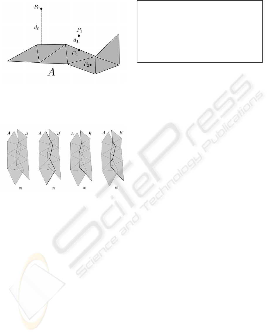
Figure 2: Three points and a patch A: distance d
0
between
P
0
and A is greater than a given threshold ε, so P
0
does not
project on A; distance d
1
between P
1
and A is lower than
ε, but the closest point C
1
is on a border edge of A, so also
P
1
does not project on A; finally, P
2
project on A, since its
distance from A is lower than ε and closest point does not
lie on border of A.
Figure 3: Two patches (a), labeled as A and B, and possible
frontiers between them; the frontier can be made of border
faces from A (b) or B (c), or it can be mixed with part of
border from A and part from B (d).
ing from the first face in the queue, we check all faces,
testing redundancy. Each face is tested once, and then
it is removed from the queue; if the face is redundant,
then it will be also removed from the original mesh,
and its neighbors will be added to Q. The process
stops when Q is empty, and all the faces involved in
the process have been tested.
2.2 Clipping
At this point, the redundant faces have been removed
from A and B and we are in a situation where there is
an overlap between the two meshes so that every face
on the border of a patch is only partially overlapping
the other patch.
Our clipping algorithm consist of two steps:
1. refine the faces on the border of the patch A until
no border edge projects on more than one face of
B;
2. remove from each face of B the part covered by a
Erosion ( Patch A, patch B){
Q = BorderOf (A) + BorderOf (B) ;
while ( ! queue . empty ( ) ) {
Face f = Q. pop ( ) ;
i f ( Redundant ( f , OtherPatch ( f ) ) ){
RemoveFromThePatch ( f ) ;
queue += Adjacents ( f ) ;
}
}
}
Figure 4: The erosion algorithm selects the lowest priority
face until there is redundancy of data.
projection and retriangulate the remain.
2.2.1 Refinement
he first step if carried out as follows. We keep a queue
B
A
of faces of A to be processed and initialize it with
the border faces of A. Then the following steps are
applied until the queue is empty.
Remove a face F
A
from B
A
, project its two border
vertices, named v
0
and v
1
, on the surface of B. Let F
0
and F
1
be the faces of B where projections of v
0
and
v
1
lie, and let e
0
the border edge between v
0
and v
1
.
Then one of the followings holds:
• F
0
and F
1
are the same face, in this case, the pro-
jection of e
0
lies completely inside the face, we
associate the face F
A
with F
0
(see Figure 5.(a)).
• F
0
is adjacent to F
1
, that is, they share an edge;
we name this edge e
S
, in this case we create a ver-
tex on the edge e
S
positioned at the closest point
of e
S
to e
0
and replace the face F
A
with two faces
as shown in Figure 5.(b), which are inserted in B
A
.
• F
0
is not adjacent to F
1
, in this case we simply
split the face F
A
along the middle point of the bor-
der edge and insert the resulting faces in B
A
(see
Figure 5.(c).
• One of the two vertices does not project on B
(see Figure 6.(a)), in this case we simply consider
the non projecting vertex, say it is v
0
as project-
ing in an ideal face of patch B passing through v
0
and process the faces as explained in the previous
cases.
• None of the vertices project, in which case there
is no action to take (see Figure 6.(b)).
In other terms, we refine the faces until the first case is
verified (see Figure 5.(c)). Note that the last two cases
always happen when only a portion of one patch over-
laps the others, while may not be encountered when
using a patch to close a hole.
GRAPP 2010 - International Conference on Computer Graphics Theory and Applications
106
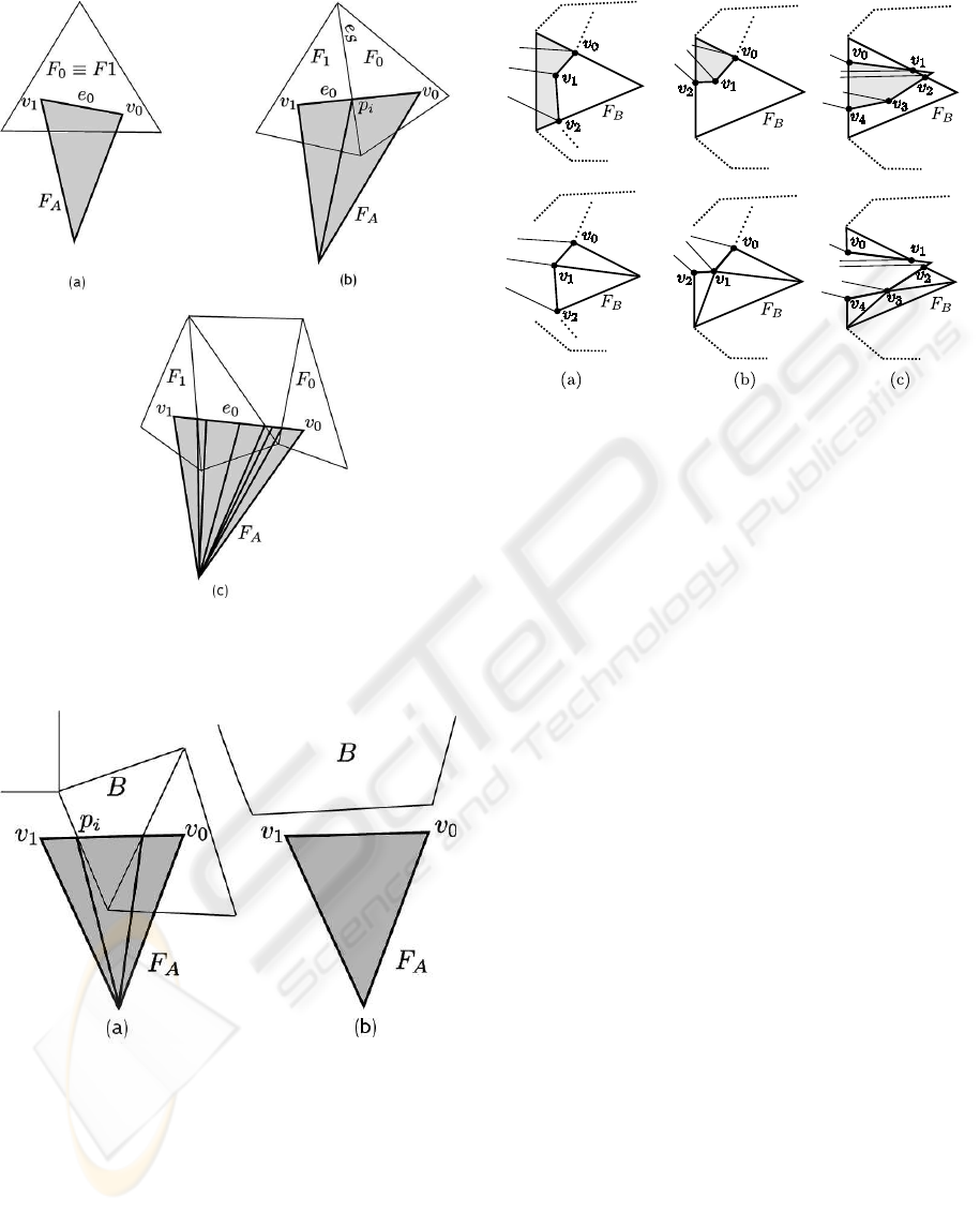
Figure 5: (a) projection of both vertices lie in one face; (b)
in two adjacent faces. (c) projections lie on non adjacent
faces: the border face is recursively split.
Figure 6: Two additional case: vertex v
1
is not projectable
on mesh, so edge is split on point p
i
, then only segment
from v
0
to p
i
is projected on B; both v
0
and v
1
are not pro-
jectable, so F
A
will not be modified.
2.2.2 Removal and Retriangulation
At this point each of the projecting faces of A will
be associated with a face of B. What we need to do
is to decompose each face of B in a part clipped by
the projection of the faces of A and a part to be retri-
angulated accordingly to such projections. As shown
Figure 7: Examples of face clipping. The polygon shaded
in gray is to be removed, the rest of face F
B
will be retrian-
gulated.
in Figure 7 for each face F
B
to clip we will have one
or more polylines with ending vertices exactly on the
edges of F
B
, which allow to separate the face in non-
clipped and clipped part. Then we only need to dis-
card the clipped parts and to retriangulate the remain-
ing polygon. Note that in rare situations we can also
have more than one remaining polygon for the same
face (see Figure 7.(c)).
2.3 Cleaning
The quality of the faces is an important part of any
reconstruction techniques. In this sense the zippering
bears a clear disadvantage since it uses a constrained
triangulation. On the other hand, we know exactly the
region of the resulting mesh where the quality of the
faces tends to be poor and may selectively filter those
parts. Furthermore, we know that the poorly shaped
faces are mostly the result of almost planar subdivi-
sion (during the refinement step) or planar retriangu-
lations (the final part of clipping).
3 EXPERIMENTAL RESULTS
In this section, we present some results of the exper-
iments conducted. For each result we also gave in-
formation about time consumed by each stage of the
algorithm. All of the experiments were performed on
a Inter Quad-Core Q9550 2.83GHz equipped with a
NVidia GeForce GTX 260 and 4,00 GB of on-board
memory. Our algorithm has been developed as a plu-
CONTROLLED AND ADAPTIVE MESH ZIPPERING
107
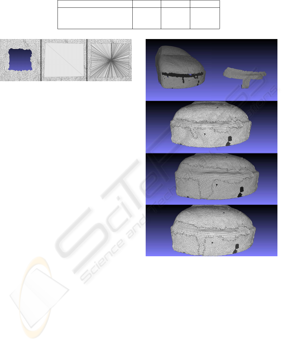
Table 1: Result table for experiment shown in Figure 9.
Criteria Erosion Clipping Cleaning
Preserving model’s face 938 ms 1018 ms 79 ms
Preserving patch’s face 1016 ms 4454 ms 89 ms
Using distance from border 962 ms 1050 ms 90 ms
Figure 8: Test case. A hole in a dense mesh (left) is cov-
ered with with a quad (center) and the algorithm produces a
conformal mesh.
gin for the MeshLab system (Cignoni et al., 2008).
Figure 9 shows a model of a car with a large missing
part and the patch that covers the missing part (top
row). We applied our algorithm with three different
criteria: by preserving the faces of the model, by pre-
serving the faces of the patch and by weighting the
faces on the base of their distance from the border,
so obtaining a clipping frontier in the middle of the
previous two. Table 1 reports the timing for the three
cases.
The most interesting experiment is the compari-
son with the Poisson Surface Reconstruction Algo-
rithm (Kazhdan et al., 2006) to merge two range maps
with 2.5M triangles each. The range maps, obtained
with a Breukmann Smartscan laser scanner1 (Breuck-
mann, 2010), are very dense (100 samples per mil-
limeter) and very well aligned. Figure 10 shows two
range maps merged using PSR (left) and the result or
our zippering algorithm (right). The bottom of the fig-
ure shows the Hausdorff distance between the two re-
sults mapped as false color on the mesh. As expected,
the result is essentially the same and the sewing re-
gions are not noticeable. However, our zippering al-
gorithm took 1m27s seconds to complete against the
6m16s of the Poisson Surface Reconstruction. Note
that the PSR is done with the original source code pro-
vided by the authors and in the same hardware setup.
4 CONCLUSIONS
We presented an improved version of the zipper-
ing algorithm for merging meshes which extends the
original version by enabling enhanced control over
the redundancy of data and supporting merging of
meshes with very different granularity. In the exam-
ples above, we presented results of merging of two
Figure 9: A large hole on the surface of a mesh and zip-
pering with three different criteria: faces from mesh are
preserved, then faces from patch are preserved and, finally,
faces are weighted using their distance from border.
different mesh, but the procedure can be easily ex-
tended in order to manage more than two meshes,
e.g. two or more patches covering a single hole, or
two or more range maps partially overlapping. Our
experiments shown that with modern range scanners
and thanks to the significant improvements made to
the scanning pipeline since the dawn of 3D scanning,
mesh zippering is back as a viable and efficient solu-
tion to merging.
GRAPP 2010 - International Conference on Computer Graphics Theory and Applications
108
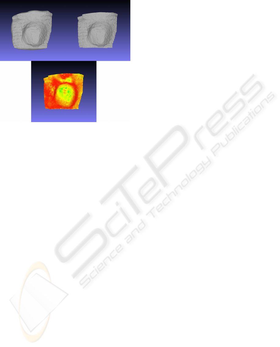
Figure 10: Poisson reconstruction, on the left, and zip-
perend range maps on the right. The bottom of the figure
shows Hausdorff distance between the two results mapped
to a ramp between red (0m) and blue(0.001m).
REFERENCES
Alexa, M., Behr, J., Cohen-Or, D., Fleishman, S., Levin, D.,
and Silva, C. T. (2001). Point set surfaces. In VIS ’01:
Proceedings of the conference on Visualization ’01,
pages 21–28, Washington, DC, USA. IEEE Computer
Society.
Bernardini, F., Mittleman, J., Rushmeier, H., Silva, C., and
Taubin, G. (1999). The ball-pivoting algorithm for
surface reconstruction. IEEE Transactions on Visual-
ization and Computer Graphics, 5:349–359.
Breuckmann (2010). Breuckmann smartscan.
http://
www.breuckmann.com
.
Cignoni, P., Callieri, M., Corsini, M., Dellepiane, M.,
Ganovelli, F., and Ranzuglia, G. (2008). MeshLab: an
Open-Source Mesh Processing Tool. In Sixth Euro-
graphics Italian Chapter Conference, pages 129–136.
Curless, B. (1999). From range scans to 3D models. Com-
puter Graphics, 33(4):38–41.
Dellepiane, M., Venturi, A., and Scopigno, R. (2009). Im-
age guided reconstruction of un-sampled data: a co-
herent filling for uncomplete cultural heritage mod-
els. In IEEE Workshop on eHeritage and Digital Art
Preservation, page In press. IEEE.
Duan, Y. and Qin, H. (2003). 2.5 d active contour for sur-
face reconstruction. Proceedings of the Eighth Inter-
national Workshop on Vision, Modeling, and Visual-
ization (VMV 2003), page 431439.
Edelsbrunner, H. and M
¨
ucke, E. P. (1994). Three-
Dimensional Alpha Shapes. ACM Transactions on
Graphics, 13:43–72.
Fiorin, V., Cignoni, P., and Scopigno, R. (2007). Out-
of-core MLS reconstruction. In Proc. of he
Ninth IASTED International Conference on Computer
Graphics and Imaging (CGIM), pages 27–34.
Guennebaud, G. and Gross, M. (2007). Algebraic point set
surfaces. ACM Transactions on Graphics, 26:23.
Hoppe, H., DeRose, T., Duchamp, T., McDonald, J., and
Stuelzle, W. (1992). Surface reconstruction from un-
organized points. In ACM Computer Graphics Proc.,
Annual Conference Series, (SIGGRAPH 92), pages
71–78.
Kazhdan, M., Bolitho, M., and Hoppe, H. (2006). Pois-
son surface reconstruction. Proceedings of the fourth
Eurographics symposium on Geometry processing,
page 70.
NextEngine (2010). Nextengine laser scanners.
http://
www.nextengine.com/
.
Ohtake, Y., Belyaev, A., Alexa, M., Turk, G., and Seidel,
H.-P. (2003). Multi-level partition of unity implicits.
ACM Transactions on Graphics, 22:463–470.
Pereira, M. G., Anderson, S., Davis, J., Ginsberg, J., Shade,
J., and Fulk, D. (2000). The Digital Michelangelo
Project: 3D Scanning of Large Statues. Proc. ACM
SIGGRAPH Conf., pp:131–144.
Shen, C., O’Brien, J. F., and Shewchuk, J. R. (2005). In-
terpolating and approximating implicit surfaces from
polygon soup. ACM SIGGRAPH 2005 Courses on -
SIGGRAPH ’05, page 204.
Turk, G. and Levoy, M. (1994). Zippered polygon
meshes from range images. ACM Computer Graph-
ics, 28:311–318.
CONTROLLED AND ADAPTIVE MESH ZIPPERING
109
