
BIDIRECTIONAL HIERARCHICAL NEURAL NETWORKS
Hebbian Learning Improves Generalization
Mohammad Saifullah, Rita Kovordanyi and Chandan Roy
Department of Computer and Information Scince, Linköping University, Linköping, Sweden
Keywords: Generalization, Image Processing, Bidirectional Hierarchical Neural Networks, Hebbian Learning, Feature
Extraction, Object Recognition.
Abstract: Visual pattern recognition is a complex problem, and it has proven difficult to achieve satisfactorily in
standard three-layer feed-forward artificial neural networks. For this reason, an increasing number of
researchers are using networks whose architecture resembles the human visual system. These biologically-
based networks are bidirectionally connected, use receptive fields, and have a hierarchical structure, with
the input layer being the largest layer, and consecutive layers getting increasingly smaller. These networks
are large and complex, and therefore run a risk of getting overfitted during learning, especially if small
training sets are used, and if the input patterns are noisy. Many data sets, such as, for example, handwritten
characters, are intrinsically noisy. The problem of overfitting is aggravated by the tendency of error-driven
learning in large networks to treat all variations in the noisy input as significant. However, there is one way
to balance off this tendency to overfit, and that is to use a mixture of learning algorithms. In this study, we
ran systematic tests on handwritten character recognition, where we compared generalization performance
using a mixture of Hebbian learning and error-driven learning with generalization performance using pure
error-driven learning. Our results indicate that injecting even a small amount of Hebbian learning, 0.01 %,
significantly improves the generalization performance of the network.
1 INTRODUCTION
Generalization is one of the most desired attributes
of any object recognition system. It is unreasonable
and impractical to present all existing instances of an
object to a recognition system for learning. A well-
designed system must be robust enough to learn the
appearance of an object from a few available
instances and to generalize the learnt response to
novel instances of the same object.
Humans are generally flexible and quite good at
generalization. For example, we can easily recognize
any legible English letter, no matter who wrote it. In
tasks such as this, we use our past knowledge of the
shape of a letter for recognizing it. This capability of
the human visual system attracts researchers to find
out the underlying mechanism of the primate visual
cortex and to emulate these mechanisms when
developing artificial object recognition systems.
The human visual system is hierarchically
organized, and has many layers. Consecutive layers
are connected in both feed forward and feedback
directions (Callaway, 2004). The interactive
property of these biological networks is nicely
captured by bidirectional hierarchical artificial
neural networks, which are considered to be
biological plausible, and are often used for
modelling human vision.
Backpropagation of error is a powerful error-
driven learning algorithm. Biologically-based forms
of backpropagation of error are therefore a good
candidate for learning algorithm that can be used in
human-like bidirectional hierarchical networks.
Error-driven learning is widely used in artificial
neural networks for image processing and object
recognition tasks. However, error driven learning in
these networks is often used to drive weight changes
on the level of individual pixels in the input image.
This technique, on the one hand helps to learn a task
very well; on the other hand, it creates a risk for
overfitting. This risk increases as the network size in
terms of number hidden layers and number of units
in each layer increases.
There are different ways to overcome the risk of
overfitting. One way is to increase the training input
to the network. But this option is not always a
feasible option due to obvious reason of limited
105
Saifullah M., Kovordanyi R. and Roy C. (2010).
BIDIRECTIONAL HIERARCHICAL NEURAL NETWORKS - Hebbian Learning Improves Generalization.
In Proceedings of the International Conference on Computer Vision Theory and Applications, pages 105-111
Copyright
c
SciTePress
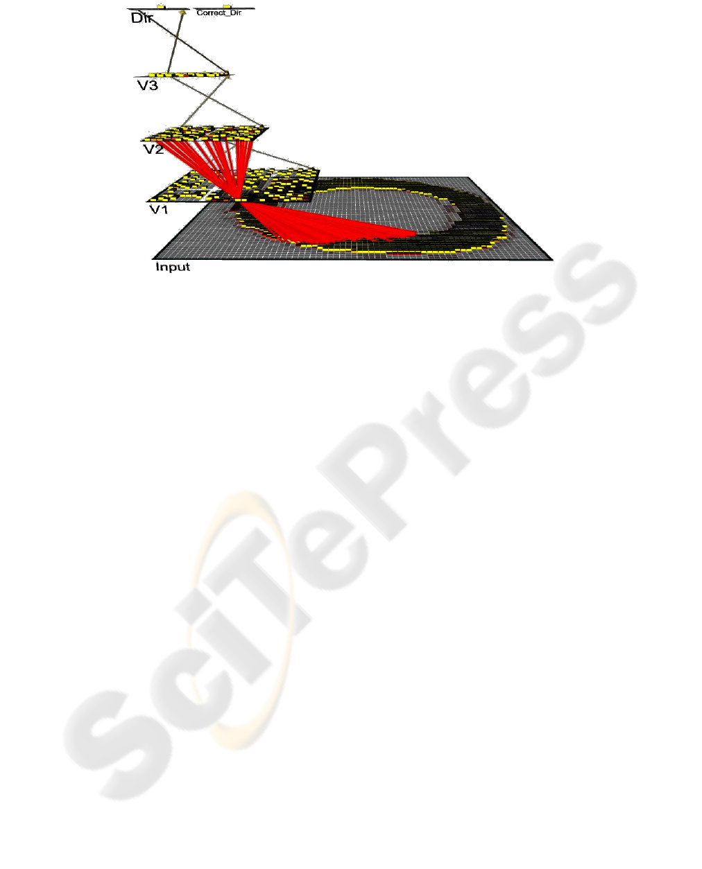
Figure 1: The bidirectional hierarchical network used for testing various learning mixes. Highlighted lines show the
connectivity pattern of a unit in layer V1. As can be seen, units in V1 received input from a limited patch of the image.
resources and time for training.
Second, one could keep down the degrees of
freedom in the network, either through careful
choice of hidden layer size and number of weights,
or by introducing a bias on weight development
during training for example, using weight decay to
kill off weak weights that tend to encode noise in the
input, or by actually pruning the network structure,
cutting off small weights.
Third, one can use a network structure that
facilitates feature extraction that is, encoding of
local features in the input (Fukushima, 1993).
Encoding of local features is necessary if the
network is to recognize novel input where individual
features are combined in a new way.
In this study we will mix amount of Hebbian
learning with the error driven learning to see how it
affect the generalization performance of the
network.
2 HIERARCHICAL NETWORKS
Hierarchical networks for image processing are
inspired by the human visual system and have been
demonstrated to be especially well suited for
extracting local features from an image (Fukushima,
2008). In hierarchical networks, the hidden layers
are selectively connected to the previous layer, so
that groups of units in layer k send signals to a
smaller number of groups in layer k+1. This
connectivity pattern will yield a hierarchical
communication structure, where contiguous patches
of the input image are processed by an array of
receiving groups in the first hidden layer. These
groups in turn project to a smaller number of groups
in the subsequent layer, and so on, until a single
group of units covers the complete input (see figure
1 for an illustration). The advantage of such a
connectivity pattern is that it forces the network to
look at local features in the input image.
A bidirectional hierarchical network is a
hierarchical network with bidirectional connection
between adjacent layers. Bidirectional networks are
quite powerful, but may also be difficult to
understand due to the relatively complex attractor
dynamics that can arise as a result of the
bidirectional connectivity.
2.1 Hebbian Learning
In its original form, Hebbian learning rewards the
co-activation of pairs of receiving and sending units,
increasing the weights of co-activated units (Hebb,
1949). In addition to this, modified Hebbian learning
rules can also decrease the weights of nodes that are
inconsistently activated, one node being activated
and the other not (O'Reilly, 2000). These modified
Hebbian learning rules turn out to capture the
statistical regularities in the input space, and will
develop a weight structure that promotes the
detection of local features in the input (McClelland,
2005).
The question is: What role does Hebbian
learning play for the generalization capability of
these networks?
Previous research suggests that Hebbian lear-
VISAPP 2010 - International Conference on Computer Vision Theory and Applications
106
ning is important for generalization in
bidirectionally connected networks (O'Reilly, 2001).
The role of Hebbian learning has, however, not been
investigated in bidirectional hierarchical networks.
Bidirectional hierarchical networks are used in
human vision and account for many important
biological vision phenomena like attention, pattern
completion, and memory (Wallis, 1997). It is
therefore motivated to investigate these networks’
learning and generalization performance.
2.2 Our Network Architecture
A bidirectional hierarchical network was developed
in Emergent (Aisa, 2008). It consists of five layers,
namely Input V1, V2, V4 and Dir (Figure 1). An
additional layer correct_dir was introduced. This
layer does not take part in actual processing of the
data, but allow us to visually compare the network’s
output with desired output. Input layer consists of
66X66 units. This layer is divided into nine
rectangular receptive fields each of size 26 X 26
with an overlap of 6 units on each side. Second layer
V1, containing 24 X 24 units, is divided into 9 equal
rectangular parts. Where as each part consists of 8 X
8 units. Each part receives input from a
corresponding receptive field from input layer. Third
layer V2 is of size 16 X 16. This layer is divided into
4 equal parts. Each part receives input from a group
of 16 X 16 units from the previous layers. Fourth
layer V3 is of size 12 X 12. It is fully connected with
the previous V2 layer. The last layer, Output layer,
contains eight units. Each represents one of the eight
English alphabets for recognition.
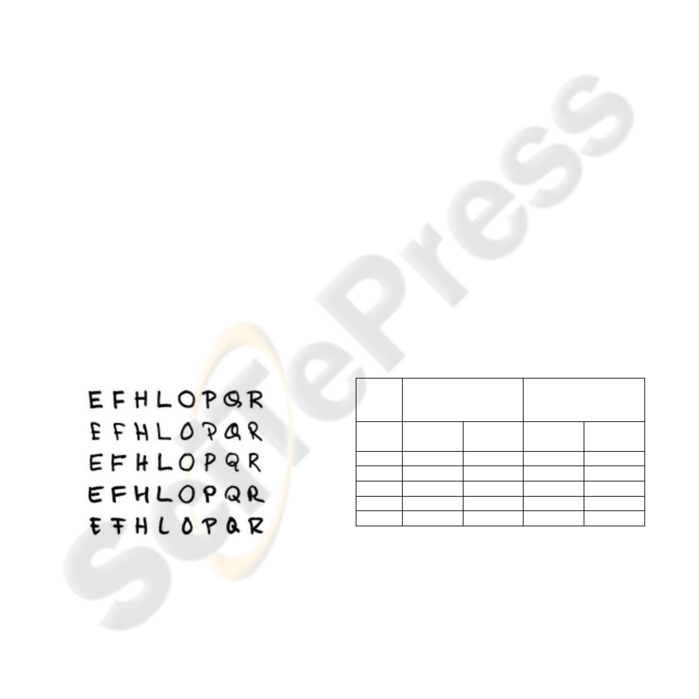
Figure 2: Data sets used for testing and training.
3 TESTING PROCEDURE
The network’s task was to recognize eight different
categories of handwritten English capital letters. The
choice of the letters was made on the basis of their
structure. We wanted to use letters that shared some
features, in order to make the categorization task
more difficult. The problem that could arise in a
badly trained network is that the constituent features
or one letter were recombined and gave rise to false
recognition of another letter. For example, letters ‘E’
and ‘H’ share the vertical line ‘I’ and horizontal
line’-’as feature. We got five different hand written
letter sets from five different persons, where as each
set consist of eight letters. The original images were
resized and shifted in four steps in eight directions,
producing about 3600 images. Out of the six set of
images, we kept aside one set of images (600
images) for testing with trained network as novel
images. From the remaining five sets, we used 75 %
of images as training the network and 25 % for
testing the trained network. In this way we wanted to
evaluate the performance of the network on trained
as well as entirely novel set of images.
We ran systematic tests of pairs of identical
networks, the only difference being the amount of
Hebbian learning in the learning mix for various
connections. For some network pairs, we used the
same learning mix for all connections. In the
particular test described here, we let the first level of
connections, going from the input layer to the first
hidden layer, V1, use 1% Hebbian learning, and let
subsequent connections use 0.1% Hebbian learning.
In contrast, for the no_Hebb version of the network,
we removed Hebbian learning from the learning mix
for all connections.
Table 1: Results from the generalization tests using both a
5% testing set reserved, i.e., excluded from the training set
(same handwriting), and a novel set of handwritten letters.
With 5% testing set
(Count error in %)
New set of 600
letters
(Count error in %)
Batch
No
No
Hebbian
Hebbian
No
Hebbian
Hebbian
1
3.16
1.33
18.5
3.9
2
1
0.66
14.16
4.1
3
1.66
0.66
20.33
11.98
4
1.66
0.66
15.33
2.03
5
1
0.76
16.16
7.04
Emergent offers a sigmoid-like activation
function, and saturating weights limited to the
interval [0, 1]. Learning in the network was based on
combination of Conditional Principal Component
Analysis, which is a Hebbian learning algorithm and
Contrastive Hebbian learning (CHL), which is a
biologically-based error-driven algorithm, an
alternative to backpropagation of error
(O'Reilly,2000):
BIDIRECTIONAL HIERARCHICAL NEURAL NETWORKS - Hebbian Learning Improves Generalization
107

CPCA:
hebb
= y
j
(x
i
− w
ij
)
(1)
x
i
= activation of sending unit i
y
j
= activation of receiving unit j
w
ij
= weight from unit i to unit j
CHL:
w
ij
= (x
i
+
y
j
+
− x
i
−
y
j
−
) =
err.
(2)
x
i
= activation of sending unit i
y
j
= activation of receiving unit j
x
+
, y
+
= act when also output clamped
x
−
, y
−
= act when only input is clamped
Learning mix:
w
ij
= c
hebb
hebb
+ (1 − c
hebb
)
err
]
(3)
= learning rate
c
hebb
= proportion of Hebbian learning
For the Hebb case we used c
hebb
= 0.01 for
connections from Input to V1 and c
hebb
= 0.001 for
all subsequent connections. For the No-Hebb case
we used c
hebb
= 0 for all connections. The low
amount of Hebbian learning is motivated by
previous experience and the fact that Hebbian
learning exerts a powerful influence on learning
(O'Reilly, 2000).
4 TEST RESULTS
We tested the network’s generalization capability in
two ways: First, by using the 5% testing set and
second by using translations (size, orientation, and
position variations) of one remaining set of alphabet
set. We recorded the number of errors and calculated
the percent errors that were made (table 1). It is clear
from the table 1 that Generalization performance of
the network improved for both 5% testing set as well
as novel set of images when we used both error
driven and Hebbian learning.
In addition to the above tests we analyzed the
weight structure developed during training using an
indirect method called activation-based receptive
field analysis. This analysis is based on the co-
activation of input-units and a particular receiving
unit. The average co-activation taken over all input
images reflects a tendency of this particular
receiving unit to react to particular forms of input.
The plots in figure 3 represent the sixty-four
units of the lower left group in V1 organized in the
same order as they appear within the layer. The plot
on the top of figure 3 shows receptive fields from
the input layer into the sixty-four units in V1. Note
that all these sixty-four units have the same
receptive field that is, they take input from the same
image-patch (marked with white squares). The
patterns in the large boxes are the weighted averages
of input patterns over the activation of respective V1
unit. Thus, input patterns that the receiving unit
became strongly activated for are represented with a
larger weight in the weighted average. The part of
the pattern in the big box which is delineated with
the small white box is the actual pattern which
appears in the receptive field of the given unit. The
plot on the bottom of figure 3 shows the projection
fields from the same units in V1 into the output
layer. Each unit-size rectangle in the projective
fields represents the average co-activation of a given
V1unit and the corresponding output unit, calculated
for the full set of input patterns. Thus, the projective
field show how strongly a given V1 unit signals
indirectly to each output category. As can be seen,
most units have developed useful feature
representations, and project to a small number of
directional units in the output layer.
4.1 Hebbian Learning Mix
Looking at the receptive field analysis for these
networks (figure 3) it can be seen that most of the
averaged patterns in the large boxes originate from a
specific character, or a few similar characters. This
indicates that the detector units are sensitive to
useful features that are part of similarly shaped
letters. This conclusion can be further verified by
looking at the projective field of the same units. For
example, the unit in the second row from the bottom
and fourth column from has learnt to specialize for
feature that is part of the letter ‘Q’. If we look at the
corresponding projective field pattern in the second
row and fourth column, the rectangle shows only a
single active unit (marked with intensive yellow).
This means that this particular unit in V1 is
indirectly) contributing to the recognition of only
one category of letters, namely the letter ‘Q’. There
are some units which are sensitive to a feature which
is part of more than one class of letters, but in a
graded fashion. For example the weighted average
pattern at the eighth row and first column is a mix of
‘Q’ and ‘O’. If we look at the corresponding
projection field, there are two output units that
receive activation from this unit, but in a graded
way. Hence, the feature that is extracted by this unit
is available in both letters. The final decision about
which output category should be activated is made
VISAPP 2010 - International Conference on Computer Vision Theory and Applications
108
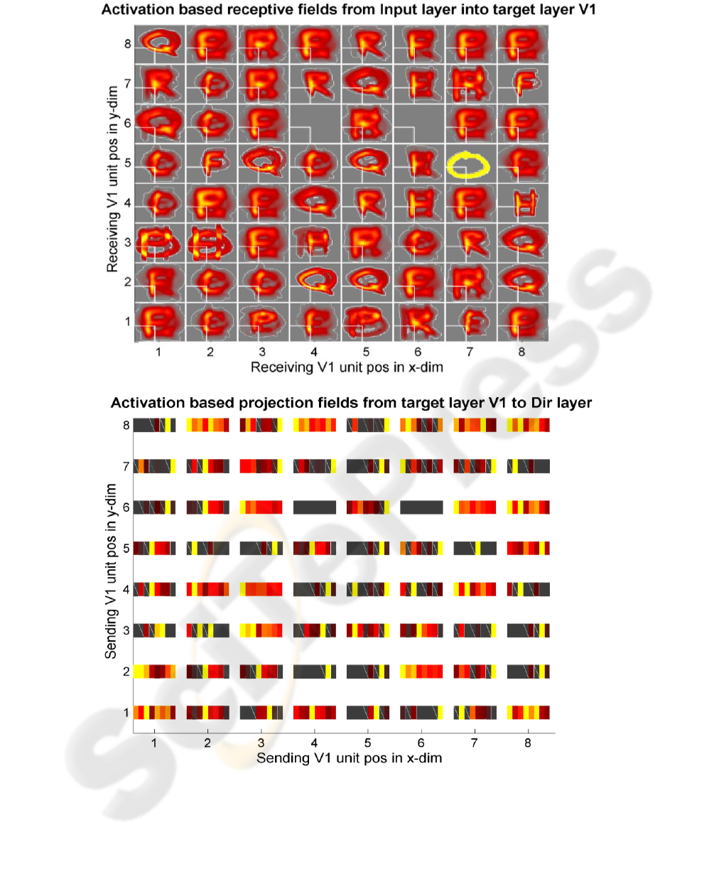
Figure 3: Activation-based receptive field and projective field analysis for layer V1, when Hebbian learning was included in
the learning mix. (top) Each big box in the plot represents the input layer and the small white box within each big box
signifies the actual receptive field for the units of a given V1 group. (bottom) Each rectangle in the plot represents the
output layer with eight units. Gray color is default background color. Pattern colors from red to yellow (dark to light)
signify the increasing activation/intensity value. Light (yellow) color represents high pixel and dark (red color) low pixel
values.
BIDIRECTIONAL HIERARCHICAL NEURAL NETWORKS - Hebbian Learning Improves Generalization
109
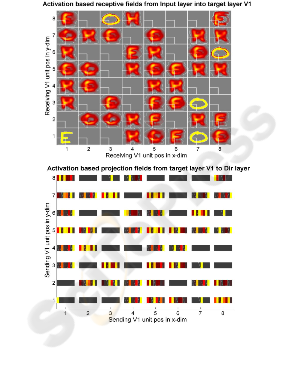
Figure 4: Activation-based receptive field and projective field analysis for layer V1, when Hebbian learning was not used
for training. The figure is organized in the same way as figure 1 and same unit group of V1 layer is used for analysis.
in later layers by combining the processing of all
other units.
Finally, we note that there are some units which
have not developed any useful features. For example
the unit in the second row and first column is not
selective for any particular class of letters. The
corresponding projective field of the unit shows that
the V1 unit in question projects to several output
VISAPP 2010 - International Conference on Computer Vision Theory and Applications
110

units, and thus is likely not to play a useful role in
the task.
4.2 Pure Error-driven Learning
Figure 4 presents the activation-based receptive field
and projective field analysis for the lower left unit
group in layer V1 when pure error-driven learning
was used for training (no Hebbian injected).
Compared to the previous figure, there are many
units here that have not developed any useful feature
representation, and project equally strongly to a
large number of output units. In addition, quite a few
units are never activated during processing. This is
probably why generalization performance suffered
when Hebbian learning was excluded from the
learning mix (Equation 3; Figures 4).
5 CONCLUSIONS
In this article, we have studied the effect of mixing
error driven and Hebbian learning in bidirectional
hierarchical networks for object recognition. Error
driven learning alone is a powerful learning
mechanism which could solve the task at hand by
learning to relate individual pixels in the input
patterns to desired perceptual categories. However,
handwritten letters are intrinsically noisy as they
contain small variations due to different
handwritings, and this increases the risk for
overfitting—especially so in large networks. Hence,
there is a risk that error-driven learning might not
give optimal generalization performance for these
networks.
We run systematic training and generalization
tests on a handwritten letter recognition task using
pure error-driven learning as compared to using a
mixture of error-driven and Hebbian learning. The
simulations indicate that mixing Hebbian and error-
driven learning can be quite successful in terms of
improving the generalization performance of
bidirectional hierarchical networks in cases when
there is much noise in the input, and an increased
risk for overfitting.
Additionally, we also believe that Hebbian
learning can be a good candidate for generic, local
feature extraction for image processing and pattern
recognition tasks. In contrast to pre-wired feature
detectors, for example, Gabor-filters, Hebbian
leaning provides a more flexible means for detecting
the underlying statistical structure of the input
patterns as it has no a priori constraints on the size or
shape of these local features.
REFERENCES
Callaway, E. M., 2004. Feedforward, feedback and
inhibitory connections in primate visual cortex. Neural
Network, 17, 625-632.
Fukushima, K., 1993. Improved generalization ability
using constrained neural network architectures,
Proceedings of the International Joint Conference on
Neural Networks, 2049-2054.
Fukushima, K., 2008. Recent advances in the
neocognitron. Neural Information Processing, Lecture
Notes In Computer Science, 1041-1050,
Berlin/Heidelberg: Springer Verlag.
Hebb, D. O., 1949. The Organization of Behavior: A
Neuropsychological Theory. New York: Wiley.
O'Reilly, R. C. and Munakata, Y., 2000. Computational
Explorations in Cognitive Neuroscience:
Understanding the Mind by Simulating the Brain.
Cambridge, MA: MIT Press.
McClelland, J., 2005. How far can you go with Hebbian
learning, and when does it lead you astray? In
Munakata, Y. and Johnson, M.H. (eds) Attention and
Performance XXI: Processes of Change in Brain and
Cognitive Development. Oxford: Oxford University
Press.
O'Reilly, R., 2001. Generalization in interactive networks:
The benefits of inhibitory competition and Hebbian
learning. Neural Computation, 13, 1199-1241.
Wallis, G. and Rolls, E. T., 1997. Invariant face and object
recognition in the visual system. Progress in
Neurobiology. 51(2), 167-194.
Aisa, B., Mingus, B. and O'Reilly, R., 2008. The emergent
neural modeling system. Neural Networks, 21, 1146-
1152.
BIDIRECTIONAL HIERARCHICAL NEURAL NETWORKS - Hebbian Learning Improves Generalization
111
