INCREMENTAL LEARNING AND VALIDATION OF SEQUENTIAL

PREDICTORS IN VIDEO BROWSING APPLICATION

David Hurych and Tom

s Svoboda

Center for Machine Perception, Department of Cybernetics, Faculty of Electrical Engineering

Czech Technical University in Prague, Karlovo N

est

ı 13, Prague, Czech Republic

Keywords:

Sequential, Linear, Predictor, Video, Browsing, Unsupervised, Incremental, Learning.

Abstract:

Loss-of-track detection (tracking validation) and automatic tracker adaptation to new object appearances are

attractive topics in computer vision. We apply very efﬁcient learnable sequential predictors in order to ad-

dress both issues. Validation is done by clustering of the sequential predictor responses. No aditional object

model for validation is needed. The paper also proposes an incremental learning procedure that accommodates

changing object appearance, which mainly improves the recall of the tracker/detector. Exemplars for the in-

cremental learning are collected automatically, no user interaction is required. The aditional training examples

are selected automatically using the tracker stability computed for each potential aditional training example.

Coupled with a sparsely applied SIFT or SURF based detector the method is employed for object localization

in videos. Our Matlab implementation scans videosequences up to eight times faster than the actual frame

rate. A standard-length movie can be thus searched through in terms of minutes.

1 INTRODUCTION

Learnable visual trackers have recently proved their

wide applicability in object tracking in video. The

tracking poses essentially two main challenges:

i) adapting to changing appearance, ii) detecting

tracker failure – loss of track. The paper addresses

both issues but contributes mainly to the adaptation

problem. We propose to solve the adaptation prob-

lem by an incremental learning, which accomodates

changing appearance whilst tracking. We also suggest

a fast method for tracking validation (i.e. loss-of-track

detection) which uses the same model as for tracking

and does not need any additional object model. The

predictor needs only a very short (seconds) ofﬂine

learning stage before the tracking starts. The track-

ing itself is then tremendously efﬁcient, much faster

than real-time.

Tracker adaptation and loss-of-track detection

have been active topics for many years. Jepson et

al. (Jepson et al., 2008) proposed WSL tracker (3

components - Wandering, Stable and Lost) - an adap-

tive appearance model which deals with partial occlu-

sion and change in object appearance. It is a wavelet-

based model, which allows to maintain a natural mea-

sure of the stability of the observed image structure

during tracking. This approach is robust and works

well with slowly changing object appearance. How-

ever, a high computational overhead precludes real-

time applications. Lim et al. (Ross et al., 2008) pro-

pose an algorithm for incremental learning and adap-

tation of low dimensional eigenspace object represen-

tation with update of the sample mean and eigenbasis.

Their approach appears to be robust to sudden illu-

mination changes and does not need ofﬂine learning

phase before tracking however, the algorithm speed

does not ﬁt our needs. For template-based track-

ers the adaptation means continuous update of the

tracked template. Tracking systems with naive up-

dates update the template after every tracking step

(Shi and Tomasi, 1994). Sub-pixel errors inherent to

each match are stored in each update and these errors

gradually accumulate resulting in the template drift-

ing off the feature. Despite this drawback, naive up-

date is still usually better choice than no update at all.

Matthews et al. in (Matthews et al., 2004) propose a

strategic update approach, which trades off mismatch

error and drift. It is a simple but effective extension of

the naive update. There are two template models kept

during the tracking. The updating template is used

for an initial alignment and the template from the ﬁrst

frame is than used in the error correction phase after

alignment. If the size of correction is too large, the

algorithm acts conservatively by preventing the tem-

467

Hurych D. and Svoboda T. (2010).

INCREMENTAL LEARNING AND VALIDATION OF SEQUENTIAL PREDICTORS IN VIDEO BROWSING APPLICATION.

In Proceedings of the International Conference on Computer Vision Theory and Applications, pages 467-474

DOI: 10.5220/0002836504670474

 SciTePress

Figure 1: Video browsing procedure.

plate to be updated from the current frame.

Recently, some authors wanted to bypass an ex-

haustive off-line learning stage. Purely on-line learn-

ing has been proposed by Ellis et al. in (Ellis

et al., 2008), where a bank of local linear predic-

tors (LLiPs), spatially disposed over the object, are

on-line learned and the appearance model of the ob-

ject is learnt on-the-ﬂy by clustering sub-sampled im-

age templates. The templates are clustered using the

medoidshift algorithm. The clusters of appearance

templates allow to identify different views or aspects

of the target and also allow to choose the bank of

LLiPs most suitable for current appearance. The al-

gorithm also evaluates the performance of particular

LLiPs. When the performance of some predictor is

too low, it is discarded and a new predictor is learned

on-line as a replacement. In comparison to our work,

we do not throw away the predictors in sequence, but

we incrementally train them with new object appear-

ances in order to improve their performance.

Our learnable and adaptive tracking method, cou-

pled with a sparsely applied SIFT (Lowe, 2004) or

SURF (Bay et al., 2006) based detector, is applied for

faster than real-time linear video browsing. The goal

is to ﬁnd all object occurrences in a movie. One of

possible solutions of video browsing task would be to

use a general object detector in every frame. As it ap-

pears (Yilmaz et al., 2006), (Murphy-Chutorian and

Trivedi, 2009), it is preferable to use a combination

of an object detector and a tracker in order to speed

up the browsing algorithm and also to increase the

true positive detections. We indeed aim at processing

rates higher than real-time which would allow almost

interactive processing of lengthy videos. Our yet pre-

liminary Matlab implementation can search through

videos up to eight times faster than the real video

frame rate.

2 LEARNING, TRACKING,

VALIDATION AND

INCREMENTAL LEARNING

User initiates the whole process by selecting a rect-

angular patch with the object of interest in one im-

Figure 2: A typical video scan process. Vertical red lines

depict frames, where the object detection was run. Red

cross means negative detection or tracking failure. Green

line shows backward and forward object tracking. Green

circle means positive object detection and yellow circle de-

picts successful validation.

age. This sample patch is artiﬁcially perturbed and

a sequential predictor is learned (Zimmermann et al.,

2009). Computation of a few SIFT or SURF object

descriptors completes the initial phase of the algo-

rithm, see Figure 1. The scanning phase of algorithm

combines predictor based tracking, its validation, and

a sparse object detection. The predictor is incremen-

tally re-trained for new object appearances. Exam-

ples for the incremental learning are selected automat-

ically with no user interaction.

The scanning phase starts with the object detec-

tion running every n−th frame (typically with the step

of 20 frames) until the ﬁrst object location is found.

The tracker starts from this frame on the detected po-

sition both in backward and forward directions. Back-

ward tracking scans frames which were skipped dur-

ing the detection phase and runs until the loss-of-track

or until it reaches the frame with last found occur-

rence of the object. Forward tracking runs until the

loss-of-track or end of sequence. The detector starts

again once the track is lost. Tracking itself is vali-

dated every m−th frame (typically every 10 frames).

The scanning procedure is depicted on Figure 2.

One object sample represents only one object ap-

pearance. The predictor is incrementally re-trained as

more examples become available from the scanning

procedure. The next iteration naturally scans only im-

ages where the object was not tracked in the preceding

iterations.

Training examples for incremental learning are se-

lected automatically. The most problematic images-

examples are actually the most useful for incremental

training of the predictor. In order to evaluate the use-

fulness of a particular example we suggest a stability

measure. The measure is based on few extra predic-

tions of the predictor on a single frame. It means,

that we let the sequential predictor track the object in

a single static image and we observe the predictors’

behavior. See Section 2.3 for more details.

The sequential linear predictor validates itself.

Naturally, an object detector may be also used to val-

idate the tracking. For example well trained face de-

tector will do the same or better job when used to val-

idate human face tracking. Motivation for using the

sequential predictor for validation is its extreme ef-

VISAPP 2010 - International Conference on Computer Vision Theory and Applications

468

ﬁciency, and robust performance. For more details

about the tracking validation, see section 2.2.

2.1 Incremental Learning of Sequential

Learnable Linear Predictor

We extend min-max learning of the Sequential learn-

able linear predictors (SLLiP) by Zimmermann et

al. (Zimmermann et al., 2009) in order to predict not

only translation but also the afﬁne deformation of the

object. Next extension is the incremental learning of

new object appearances. The predictor essentially es-

timates motion and deformation parameters directly

from image intensities. It requires an ofﬂine learning

stage before the tracking starts. The learning stage

consists of generating exemplars and estimation of re-

gression functions. We use 2 SLLiPs - ﬁrst for 2D mo-

tion estimation (2 parameters) and second for afﬁne

warp estimation (4 parameters). We have experimen-

tally veriﬁed that, especially for low number of train-

ing examples, this conﬁguration is more stable than

using just one SLLiP to predict all 6 parameters at

once. Using smaller training set decreases the nec-

essary learning time which is important for the fore-

seen applications. Because of speed we opted for least

squares learning of SLLiPs similarly, as suggested by

Zimmermann et al. in their any-time learning algo-

rithm (Zimmermann et al., 2009).

Let denote the translation parameters vector t

[∆x,∆y]

estimated by the ﬁrst SLLiP, and the afﬁne

warp is parameterized by the parameters vector t

[α,β,∆s

,∆s

]

which is estimated by the second

SLLiP. The 2 × 2 afﬁne warp matrix A is computed

A = R

−β

, (1)

where R are standard 2D rotation matrices parameter-

ized by the angles α,β and S is the scale matrix

S =



1 + ∆s

0 1 + ∆s



. (2)

Than the image point x = [x,y]

is transformed be-

tween two consecutive images using estimated pa-

rameters accordingly

= Ax + t

(3)

= R

−β

x + t

Tracking, learning and incremental learning will

be explained for SLLiP with general parameters vec-

tor t. Equations are valid for both SLLiPs, which we

use. SLLiP is simply a sequence of linear predic-

tors. Predictors in this sequence estimate the param-

eters one after each other (see equation 4), thus each

improving the result of previous predictor estimation

and lowering the error of estimation. SLLiP tracks

according to

= H

I (X

) (4)

= H

I (t

◦ X

)

= H

I (t

◦ X

)

t = 

(i=1,...,k)

where I is current image and X is a set of 2D co-

ordinates spread over the the object patch - it is called

support set. I (X ) is a vector of image intensities col-

lected at image coordinates X. Operation ◦ means

transformation of support set points using Equation 3,

i.e. aligning the support set to ﬁt the object using pa-

rameters estimated by the previous predictor in the se-

quence. Final result of the prediction is vector t which

combines results of all predictions in the sequence.

The model θ

for SLLiP is formed by the sequence

of predictors θ

}

{

}

,...,

{

Matrices H

,...,H

are linear regression matrices

which are learned from training data.

In our algorithm, the SLLiP is learned from one

image only and it is incrementally (re-)learned after

each video scan. A few thousands of training ex-

amples are artiﬁcially generated from the ﬁrst image

using random perturbations of parameters in vector

t, warping the support set accordingly and collect-

ing the image intensities. The column vectors of col-

lected image intensities are stored in matrix D

and

perturbed parameters in matrix T

columnwise. Each

regression matrix in SLLiP is trained using the least

squares method H

= T





−1

. The initial learn-

ing phase takes 5 or 6 seconds on a standard PC.

More images (around 400) are selected for

incremental learning from all images gathered during

last scanning iteration. From each of the additional

exemplars 10 training examples are generated. This

procedure provides additional 4000 training examples

after each particular video scan. It is worth to note

that this process is completely automatic, no user

interaction is required. Incremental learning com-

prises update of regression matrices H

,i = 1,...,k.

An efﬁcient way of updating regression matrices was

proposed by Hinterstoisser et al. in (Hinterstoisser

et al., 2008).

Each regression matrix H

may be computed alter-

natively

= Y

, (5)

where Y

= T

and Z





−1

. Lets denote

, where j indexes the training examples. New

INCREMENTAL LEARNING AND VALIDATION OF SEQUENTIAL PREDICTORS IN VIDEO BROWSING

APPLICATION

469

training example d = I (X) with parameters t is incor-

porated into the predictor as follows

j+1

= Y

+ td

(6)

j+1

= Z

−

1 + d

After updating matrices Y

and Z

we may also update

the regression matrices H

using equation 5. For more

details about incremental learning see (Hinterstoisser

et al., 2008).

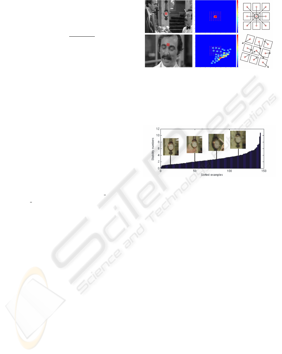
2.2 Validation by Voting

To validate the tracking (i.e. detecting loss-of-track)

we use the same sequential linear predictor as for

tracking. We utilize the fact that the predictor is

trained to point to the center of this object when ini-

tialized in a close neighborhood. On the contrary,

when initialized on the background, the estimation of

2D motion is expected to be random.

We initialize the predictor several times on a regu-

lar grid (validation grid - depicted by red crosses in

Figure 3) in the close neighborhood of current po-

sition of the tracker. The close neighborhood is de-

ﬁned as 2D motion range, for which the predictor was

trained. In our case the range is ±(patch width/4)

and ±(patch height/4). The validation grid is de-

formed according to estimated parameters. Then we

observe the 2D vectors, which should point to the cen-

ter of the object, i.e. current tracker position in the

image. When all (or sufﬁcient number of) the vec-

tors point to the same pixel, which is also the current

tracker position, we consider the tracker to be on its

track. Otherwise, when the 2D vectors are pointing to

some random directions, we say that the track is lost,

see Figure 3.

A threshold value is needed in order to recognize

if the sum of votes, which point to the center of object,

is big enough to pass the validation. The threshold is

set automatically from examples collected during the

video scan. At ﬁrst iteration, when no threshold is

available, ﬁrst few (tens) validations are done by the

object detector and SLLiP simultaneously. When the

detector votes for positive validation, also the current

sum of votes is taken as positive example. Negative

examples (sums of votes) are collected by placing the

validation grid on other parts of the image, where the

object does not appear. Gaussian distributions are ﬁt-

ted into positive and negative examples and the clas-

sical Bayes threshold is found. Both negative and

positive cases are considered to appear equally likely.

In subsequent iterations, the additional training exam-

ples are also used for threshold update.

Figure 3: Example of predictor validation. The ﬁrst row

shows successful validation of clock tracking. Second row

shows loss-of-track caused by a sudden scene change just

after a video cut. Red crosses depict pixels, where the pre-

dictor was initialized - validation grid. Right column of

pictures illustrates the idea of validation using linear pre-

dictors and the middle column shows the collected votes for

the center of the object in normalized space.

Figure 4: Blue bars depict sorted stability numbers. The

left most clock image was used for predictor training. The

other occurrences obtained during tracking were automat-

ically evaluated as more difﬁcult examples for the tracker.

Clearly, the higher stability measure, the more difﬁcult case

for the predictor.

2.3 Stability Measure and Examples

Selection for the Incremental

Learning

Selecting only relevant examples for training may

speed up the learning as well as increase the perfor-

mance. Clearly relevant examples are those which

contain the object but were not included in the pre-

vious training examples. The predictor has of course

problems to handle new object appearances and it is

likely, that it will loose the track. It is reasonable

to presume, that these new difﬁcult (and useful) ex-

amples should appear near frames, where the loss-of-

track was detected. We need to examine the object oc-

currences, which appeared near loss-of-track frames,

in order to capture the most interesting examples for

incremental learning. We propose the stability mea-

sure for evaluation of these object occurrences.

When we let the predictor track object on a sin-

gle frame, we would expect the tracker to stay still in

objects’ position with no additional change of param-

eters. However, due to inherent noise in the data the

VISAPP 2010 - International Conference on Computer Vision Theory and Applications

470

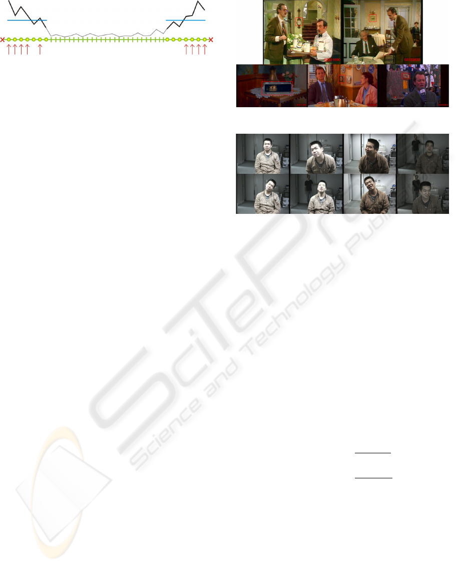
Figure 5: Illustration of examples selection for incremental

learning. Green line depicts one interval - subsequence of

video frames, where the object was found during scanning

procedure. Only few images near the beginning and end

of the interval are examined. Yellow circles mean success-

ful validation. The black curve depicts computed stability

measure on particular frames. The examples with stability

number above the blue line are considered as useful for in-

cremental learning. Selected examples are marked by red

arrows.

predictor predicts non-zero parameters even when ini-

tiated on the correct position. The parameters changes

are accumulated and their sum-of-squares is com-

puted after 10 tracking steps. Let t be the vector of

parameters estimated during tracking and p

vector of

parameters obtained in i−th step of this single frame

tracking. The stability number s for current frame is

computed as s =

∑

i=1

k t − p

. Clearly, the higher

value the more difﬁcult example, see Figure 4. Pa-

rameters changes in both vectors are made relative to

particular ranges, in order to obtain stability number,

which is not dependent on different parameters units.

Using this stability number we may evaluate how use-

ful (difﬁcult) is the examined object occurrence.

We use this stability number to select a ﬁxed num-

ber of additional training examples from each inter-

val obtained during one video scan. Each interval is

a continuous subsequence of images from the whole

video sequence (one interval is depicted as a green

line in Figure 2).

We search for the best additional training exam-

ples near the borders of each interval. We go through

ﬁxed number of images from the start of the interval

forwards and backwards from the end of the interval,

while computing the stability number on tracker po-

sitions. Finally, the algorithm selects the examples

with high stability number for incremental learning.

Tracker positions in these images have also passed

validation and we expect them to be well aligned to

the object. The procedure of examples selection is

depicted in Figure 5.

3 EXPERIMENTS

Real sequences used in experiments includes an

episode from Fawlty Towers series (33 minutes,

720 × 576), and Groundhog Day movie (1 hour 37

minutes, 640 × 384). Several objects were tested, see

Figure 6: Tested objects are marked with red rectangle.

Figure 7: Here you may see examples of human face data

used in experiment. All images are extracted from one

video sequence. Note signiﬁcant deformations and varia-

tions in illumination.

Figure 6. The ground truth data for the Groundhog

Day were kindly provided by Josef

Sivic and they are

the same as in (Sivic and Zisserman, 2009). We have

manually labeled ground truth for two tested objects

in Fawlty Towers. Third tested sequence captures a

human moving in front of the camera (2 minutes 50

seconds, 640 × 480), see Figure 7. Matlab implemen-

tation of the algorithm was used for all experiments.

SIFT and SURF object detectors are publicly avail-

able MEX implementations. Mostly, the standard pre-

cision and recall are used to evaluate the results. Let

T P denote the true positives, FP denote the false pos-

itives and FN denote the false negatives. Than the

precision and recall are computed accordingly

precision =

T P

T P + FP

(7)

recall =

T P

T P + FN

. (8)

The experiments are organized as follows. The ﬁrst

experiment (Section 3.1) shows the effect of incre-

mental learning on resulting precision and recall. In

Section 3.2 we evaluate the overall performance of

the algorithm. Next we compare tracking validation

by SIFT and by SLLiP. Finally Table 3, Table 4 and

Table 5 show comparison of SIFT detection in every

frame with one iteration of our algorithm.

INCREMENTAL LEARNING AND VALIDATION OF SEQUENTIAL PREDICTORS IN VIDEO BROWSING

APPLICATION

471

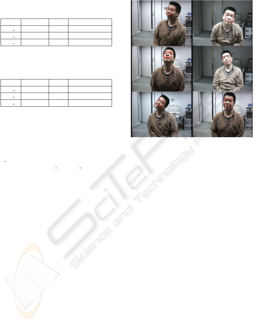
Table 1: Incremental learning evaluation for the clock ob-

ject from the Fawlty towers episode. The video scan was

running 76 frames per second in average.

precision recall cumulative time

iter 0 0.86 0.61 13 min 42 sec

iter 1 0.81 0.63 23 min 18 sec

iter 2 0.81 0.64 32 min 21 sec

Table 2: Incremental learning evaluation for human face.

The ﬁrst iteration of video scan was running 21 frames per

second in average. Browsing time was increased by using

the face detector instead of SURF.

precision recall cumulative time

iter 0 0.99 0.70 4 min 5 sec

iter 1 0.98 0.79 5 min 2 sec

iter 2 0.98 0.81 5 min 27 sec

3.1 Incremental Learning Evaluation

This experiment shows the improvement gained by

the automatic incremental learning. At ﬁrst we run

one iteration of video scan using sequential predic-

tor trained on one image only (in Table 1 denoted as

iter 0). Next, we evaluate results after ﬁrst and second

incremental learning (iter 1 and iter 2). Two objects

were tested. First was the picture object in Fawlty

Towers video (see Figure 6 top right image). The

SURF based detector was used for picture detection

with step n = 20 and sequential predictor for valida-

tion with step m = 10. Incremental learning improves

the recall while keeping high precision, see Table 1.

Second tested object was a human face (see Fig-

ure 7). In this case the object was difﬁcult to track

with SLLiP learned only from one image, because

the appearance of the face changed signiﬁcantly dur-

ing the sequence. The lighting conditions were chal-

lenging and the human face undergoes various rota-

tions and scale changes. We have chosen this se-

quence in combination with the face detector (instead

of SIFT/SURF) to see how the incremental learning

helps to improve tracking results on complex non-

rigid object. In this case incremental learning also

improved the performance of the tracker. See Table 2

for results.

The high precision obtained in the face experiment

was caused by ﬂawless face detection, which did not

return any false positive. You may see a few images

of SLLiP tracker aligned on human face on Figure 8.

3.2 Results of Detection and Tracking

One iteration of the algorithm in Fawlty Towers se-

ries runs 3−times faster than real-time and more than

Figure 8: Examples of face tracking results. Red rectangle

depicts SLLiP tracker aligned on human face.

8−times faster for the Groundhog Day movie. The

detector was run every n = 20 frames and valida-

tion every m = 10 frames while tracking. In the se-

quence with human face the browsing time was al-

most twice the real-time, even for detection step n =

40. It was caused by the face detector which runs

much slower than SURF. The difference in browsing

times in Fawlty Towers and Groundhog Day is caused

mainly by the different video resolution. Processing

of higher resolution images and more complex scenes

is slown down by the object detector. Even shorter

browsing times may be achieved by increasing the de-

tection interval n. Selecting the right interval depends

on our expectation of the shortest time interval, where

the object may appear. Reasonable values for detec-

tion interval are between 20 and 60 frames. Increas-

ing the validation interval m to more than 10 generates

more false positives and since the validation runs very

fast, it is not necessary to validate with a bigger step.

Next we compare the performance of predictor

validation with SIFT validation. The average time of

one SIFT validation was 179 milliseconds and aver-

age time of one predictor validation was 33 millisec-

onds. The resulting recall of video browsing for clock

object was 0.58 with SIFT and 0.61 with predictor

validation, while the precision was 0.9 for SIFT val-

idation and 0.86 for SLLiP validation. Recall for the

picture object was 0.94 with SIFT validation and 0.95

with predictor, while the precision was 0.84 for both.

Predictor validation gives comparable precision and

VISAPP 2010 - International Conference on Computer Vision Theory and Applications

472

Table 3: Comparison of SIFT object detection only and one

iteration of our algorithm on Fawlty Towers - clock and pic-

ture.

clock (FT) picture

SIFT detector on every frame - without tracking

browsing time 32 h. 56 m. 33 h. 29 m.

scanning speed (fps) 0.4 0.4

obtained occurrences 2440 2140

true positives 2411 1996

false positives 29 144

precision 0.99 0.93

recall 0.43 0.89

SURF detect., SLLiP track. and valid.

browsing time 13 m. 42 s. 11 m. 40 s.

scanning speed (fps) 61 71

obtained occurrences 4026 2520

true positives 3462 2131

false positives 564 389

precision 0.86 0.85

recall 0.61 0.95

Table 4: Comparison of SIFT object detection only and one

iteration of our algorithm on Groundhog Day - alarm clock

and clock.

alarm clock clock

(GhD)

SIFT detector on every frame - without tracking

browsing time 48 h. 43 m. 48 h.

13 m.

scanning speed (fps) 0.8 0.8

obtained occurrences 1888 855

true positives 1811 801

false positives 77 54

precision 0.96 0.94

recall 0.37 0.29

SURF detect., SLLiP track. and valid.

browsing time 16 m. 46 s. 12 m.

48 s.

scanning speed (fps) 144 189

obtained occurrences 1345 2034

true positives 1125 1520

false positives 220 514

precision 0.84 0.75

recall 0.23 0.55

recall in much shorter time, which also saves time in

the whole scanning iteration. Tables 3, 4 and 5 show

the results for 5 tested objects obtained in one scan-

ning iteration. The results of the video browsing al-

gorithm are compared to the results produced by the

SIFT detector only.

SURF detection on every frame was tested too, but

the results contained large number of false positives.

Table 5: Comparison of SIFT object detection only and one

iteration of our algorithm on Groundhog Day - PHIL sign.

PHIL sign

SIFT detector on every frame - without tracking

browsing time 48 h. 7 m.

scanning speed (fps) 0.8

obtained occurrences 2597

true positives 2293

false positives 304

precision 0.88

recall 0.72

SURF detect., SLLiP track. and valid.

browsing time 15 m. 15 s.

scanning speed (fps) 159

obtained occurrences 4038

true positives 2361

false positives 1677

precision 0.58

recall 0.74

Recall was comparable to SIFT detector, but preci-

sion was very low. We are using the SURF detector

because it runs much faster than SIFT, but we need to

use predictor validation after every positive detection

because of the large number of false positives. The

results show that even after a single iteration the al-

gorithm gives results comparable with SIFT detection

only.

4 CONCLUSIONS

We have shown that an incremental learning of se-

quential predictor signiﬁcantly improves its robust-

ness. It increases the recall while keeping high preci-

sion. Proposed method for collecting additional train-

ing examples is completely automatic and requires

no user interaction. Stability number well describes

the condition of the tracker on particular image and

prooves to be good criteria for training examples se-

lection. Validation by clustering SLLiP responses

works reliably and very fast.

When coupled with a sparsely applied object de-

tector the system can search for objects through

videos several times faster than real time despite the

current rather preliminary Matlab implementation.

The complete system for video browsing works very

well with simple objects. Performance for more com-

plex 3D objects (when using SIFT/SURF for detec-

tion) are not yet entirely satisfactory. It is mainly the

detector that hinders the recognition rate. The tracker

itself may be incrementally learned for new appear-

ances of the object and it works better with every it-

eration. This was veriﬁed on face tracking where a

INCREMENTAL LEARNING AND VALIDATION OF SEQUENTIAL PREDICTORS IN VIDEO BROWSING

APPLICATION

473

robust face detector was applied. We plan to extend

the sequential predictor in a way that would allow its

application as a detector.

REFERENCES

Bay, H., Ess, A., Tuytelaars, T., and Van Gool, L. (2006).

Speeded-up robust features. In Proceedings of IEEE

European Conference on Computer Vision, pages

404–417.

Ellis, L., Matas, J., and Bowden, R. (2008). On-line learn-

ing and partitioning of linear displacement predictors

for tracking. In Proceedings of the 19th British Ma-

chine Vision Conference, pages 33–42.

Hinterstoisser, S., Benhimane, S., Navab, N., Fua, P., and

Lepetit, V. (2008). Online learning of patch perspec-

tive rectiﬁcation for efﬁcient object detection. In Con-

ference on Computer Vision and Pattern Recognition,

pages 1–8.

Jepson, A., Fleet, D., and El-Maraghi, T. (2008). Robust on-

line appearance models for visual tracking. In IEEE

Conference on Computer Vision and Pattern Recogni-

tion, volume 1, pages 415–422.

Lowe, D. (2004). Distinctive image features from scale-

invariant keypoints. International Journal on Com-

puter Vision, 60(2):91–110.

Matthews, I., Ishikawa, T., and Baker, S. (2004). The tem-

plate update problem. IEEE Transactions on Pattern

Analysis and Machine Intelligence, 26(6):810–815.

Murphy-Chutorian, E. and Trivedi, M. (2009). Head pose

estimation in computer vision: A survey. IEEE Trans-

actions on Pattern Analysis and Machine Intelligence,

31(4):607–626.

Ross, D., Lim, J., Lin, R., and Yang, M. (2008). Incremen-

tal learning for robust visual tracking. International

Journal of Computer Vision, 77(1-3):125–141.

Shi, J. and Tomasi, C. (1994). Good features to track. In

Proceedings of IEEE Computer Society Conference

on Computer Vision and Pattern Recognition, pages

593–600.

Sivic, J. and Zisserman, A. (2009). Efﬁcient visual search

of videos cast as text retrieval. IEEE Transac-

tions on Pattern Analysis and Machine Intelligence,

31(4):591–606.

Yilmaz, A., Javed, O., and Shah, M. (2006). Object track-

ing: A survey. ACM Computing Surveys (CSUR),

38(4):13–36.

Zimmermann, K., Svoboda, T., and Matas, J. (2009). Any-

time learning for the NoSLLiP tracker. Image and

Vision Computing, Special Issue: Perception Action

Learning, 27(11):1695–1701.

VISAPP 2010 - International Conference on Computer Vision Theory and Applications

474