RELIEF MAPPING ON CUBIC CELL COMPLEXES

Karl Apaza and Carlos Andujar

MOVING Group, Universitat Politecnica de Catalunya, Barcelona, Spain

Keywords:

Displacement mapping, Relief mapping, GPU raycasting, Quadrilateral parameterization.

Abstract:

In this paper we present an algorithm for parameterizing arbitrary surfaces onto a quadrilateral domain deﬁned

by a collection of cubic cells. The parameterization inside each cell is implicit and thus requires storing no

texture coordinates. Based upon this parameterization, we propose a uniﬁed representation of geometric and

appearance information of complex models. The representation consists of a set of cubic cells (providing a

coarse representation of the object) together with a collection of distance maps (encoding ﬁne geometric detail

inside each cell). Our new representation has similar uses than geometry images, but it requires storing a single

distance value per texel instead of full vertex coordinates. When combined with color and normal maps, our

representation can be used to render an approximation of the model through an output-sensitive relief mapping

algorithm, thus being specially amenable for GPU raytracing.

1 INTRODUCTION

During the last few decades much research effort

has been devoted to build parameterizations between

polygonal meshes and a variety of domains, includ-

ing planar regions, triangular or quadrilateral meshes,

polycubes and spheres. The parameterization liter-

ature has focused mainly on minimizing distortion,

guaranteeing global bijectivity, and producing seam-

less parameterizations for complex surfaces. With

very few exceptions, parameterization methods for

computer graphics compute piecewise linear map-

pings that must be encoded explicitly, typically by as-

sociating a pair of texture coordinates (u, v) to each

vertex. The explicit nature of these parameterizations

makes them non-reversible, i.e. computing the point

in the mesh represented by a point (u, v) in parame-

ter space is a costly operation, unless additional data

structures are used (García and Patow, 2008). One no-

table exception are Geometry Images (Gu et al., 2002;

Losasso et al., 2003), which allow representing geo-

metric and appearance details such as color/normal

data as separate 2D arrays, all of them sharing the

same implicit surface parametrization and thus requir-

ing no texture coordinates.

In this paper we present a method to deﬁne

projection-based parameterizations of arbitrary sur-

face meshes onto a quadrilateral domain formed by a

subset of the faces of the cubic cells intersected by the

mesh (Figure 1). The resulting parameterizations are

(a) (b) (c) (d)

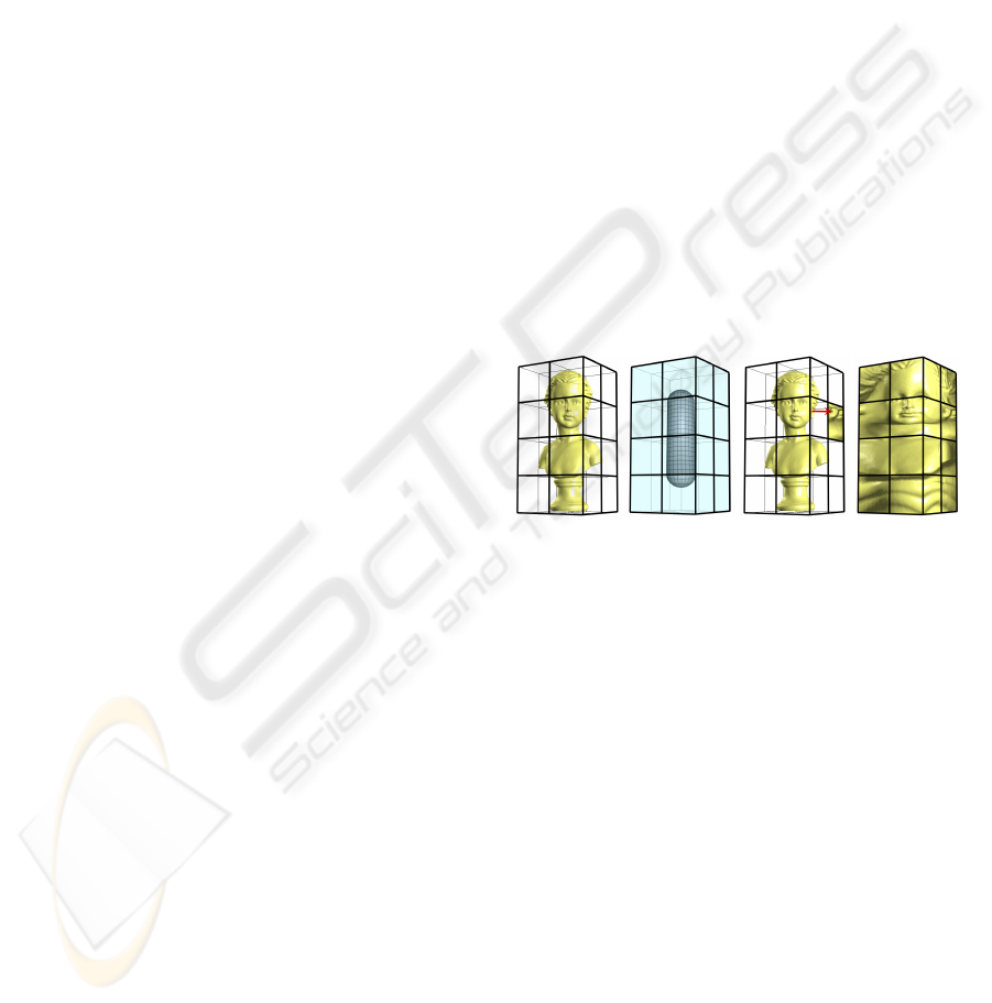
Figure 1: Overview of our approach: (a) set of cells inter-

sected by the surface mesh; (b) the direction of projection is

deﬁned by the normals of the shown surface; (c) each point

inside the cells is mapped onto a point on the external faces;

(d) mesh projected onto the external faces.

implicit and allow representing geometric and appear-

ance details using a collection of 2D arrays. Unlike

geometry images though, points (u, v) on our quadri-

lateral domain have associated a point P

= (x

)

in 3D space (on the face of a cubic cell). This fact,

along with a projection-based parameterization, al-

lows (a) encoding the coordinates of surface points

P = (x, y, z) with a single distance value ||P − P

|| in-

stead of storing global (x,y, z) coordinates in the 2D

array, and (b) computing quickly the intersection of

arbitrary rays with the mesh implicitly encoded by the

above distance maps.

Since we target GPU-based construction and ren-

dering algorithms, we restrict ourselves to easily in-

vertible, implicit projections. Given a point (u,v) on

the domain, we can easily compute the direction to-

wards the mesh point mapped to (u,v).

181

Apaza K. and Andujar C. (2010).

RELIEF MAPPING ON CUBIC CELL COMPLEXES.

In Proceedings of the International Conference on Computer Graphics Theory and Applications, pages 181-189

DOI: 10.5220/0002837001810189

 SciTePress

We use four different projection types (parallel,

perspective, axial and planar) which are chosen on

a cell-basis, according to the local neighborhood of

the cell. These projections map any point (x, y,z) in-

side the cubic cell onto a point (x

) on one of its

faces, which in turn can be expressed in local coordi-

nates (u,v) inside the face, see Figure 1(c).

Given an arbitrary surface mesh, we compute a

set of cubic cells and, using the implicit parameteri-

zation, we sample the input mesh to ﬁll in the 2D ar-

rays with attributes such as distance, normal and color

data. Each attribute is stored as an array texture. This

provides a uniﬁed representation of the surface mesh

which allows extracting a level-of-detail approxima-

tion of the original surface. Like geometry images,

our representation can be rendered using a geometry-

based approach suitable for rasterization-based visu-

alization, which involves unprojecting each texel us-

ing the implicit projection and the stored distance

value. Moreover, a unique feature of our represen-

tation is that it is amenable for raycasting rendering,

using a GPU-based algorithm with a pattern similar to

that of relief mapping algorithms. This last rendering

approach makes our representation specially suitable

for raytracing in the GPU.

The rest of the paper is organized as follows.

Section 2 reviews previous work on implicit pa-

rameterizations and relief mapping techniques. Our

projection-based parameterization and the way we

use it to construct and render detailed meshes are dis-

cussed in Section 3. Section 4 discusses our results

on several test models. Finally, Section 5 provides

concluding remarks and future work.

2 PREVIOUS WORK

In recent years a number of methods for parameter-

izing meshes have been proposed, targeting multiple

parameter domains and focusing on different param-

eterization properties such as minimizing distortion

and guaranteeing global bijectivity. Most methods

developed so far target a planar domain and thus re-

quire cutting the mesh into disk-like charts to avoid

excessive distortions and to make the topology of the

mesh compatible to that of the domain (see (Floater

and Hormann, 2005; Sheffer et al., 2006) for a recent

survey). Parameterizations onto more complex do-

mains such as triangle or quadrilateral meshes avoid

cutting the mesh and thus provide seamless param-

eterizations. A popular base domain are simplicial

complexes obtained e.g. by just simplifying the orig-

inal triangle mesh (see e.g. (Lee et al., 1998; Guskov

et al., 2000; Praun et al., 2001; Purnomo et al., 2004)),

allowing each vertex of the original mesh to be rep-

resented with barycentric coordinates inside a ver-

tex, edge, or face of the base domain. Some re-

cent approaches target quadrilateral instead of trian-

gle meshes (Tarini et al., 2004; Dong et al., 2006).

Polycube maps (Tarini et al., 2004) use a polycube

(set of axis-aligned unit cubes attached face to face)

as parameter domain. Each vertex of the mesh is

assigned a 3D texture position (a point on the sur-

face of the polycube) from which a simple mapping

is used to look up the texture information from the

2D texture domain. Construction of the parameteri-

zation involves (a) ﬁnding a proper polycube roughly

resembling the shape of the given mesh, (b) warping

the surface of the polycube so as to roughly align it

with the surface mesh, (c) projecting each mesh ver-

tex onto the warped polycube along its normal direc-

tion, (d) applying the inverse warp function to the pro-

jected vertices, and (e) optimizing the texture posi-

tions by an iterative process. Unfortunately, no auto-

matic procedure is given for steps (a) and (b), which

are done manually. Our approach also targets a do-

main formed by axis-aligned quadrilateral faces, but

differs from polycube maps in two key points: our

parameterization is implicit and thus does not require

storing texture coordinates, and it is easily invertible

and thus it is amenable to raycasting rendering. Gu et

al. (2002) propose to remesh an arbitrary surface onto

a completely regular structure called Geometry Im-

age which captures geometry as a simple 2D array of

quantized point coordinates. Other surface attributes

like normals and colors can be stored in similar 2D ar-

rays using the same implicit surface parametrization.

Geometry images are built cutting the mesh and pa-

rameterizing the resulting single chart onto a square.

Geometry images have been shown to have numerous

applications including remeshing, level-of-detail ren-

dering and compression. Our representation has simi-

lar uses than geometry images, although construction

is much simpler and requires encoding only distance

values instead of full vertex coordinates. Solid tex-

tures (Perlin, 1985; Peachey, 1985) avoid the param-

eterization problem by deﬁning the texture inside a

volume enclosing the object and using directly the 3D

position of surface points as texture coordinates. Oc-

tree textures (Benson and Davis, 2002) strive to re-

duce space overhead through an adaptive subdivision

of the volume enclosing the object. Although octree

textures are amenable for GPU decoding (Lefebvre

et al., 2005), a subdivision up to texel level (each

octree leaf representing a single RGB value) causes

many unused entries in its nodes, thus limiting the

maximum achievable resolution.

Space overhead grows even further when using N

GRAPP 2010 - International Conference on Computer Graphics Theory and Applications

182

trees or page tables to reduce the number of texture in-

directions (Lefebvre et al., 2005; Lefohn et al., 2006).

TileTrees (Lefebvre and Dachsbacher, 2007) also rely

on an octree enclosing the surface to be textured, but

instead of storing a single color value at the leaves,

square texture tiles are mapped onto leaf faces. Re-

sulting tiles are compactly stored into a regular 2D

texture. During rendering, each surface point is pro-

jected onto one of the six leaf faces, depending on sur-

face orientation. The resulting texture has little distor-

tion and is seamlessly interpolated over smooth sur-

faces. We also use projection onto cell faces, but our

work differs from TileTrees in two key aspects. On

the one hand, we do not restrict ourselves to parallel

projection; we also use perspective and axial projec-

tions whenever appropriate. On the other hand, our

approach is suitable for encoding geometry as dis-

placement maps. Note that this does not apply to Tile-

Trees because determining the face a surface point P

inside a cell must be projected onto requires knowl-

edge about both the P coordinates and its normal vec-

tor.

Relief mapping (Policarpo et al., 2005) has been

shown to be extremely useful as a compact represen-

tation of highly detailed 3D models. All the neces-

sary information for adding surface details to polyg-

onal surfaces is stored in RGBA textures, with the

alpha channel storing quantized depth values. The

technique uses an inverse formulation based on a ray-

heightﬁeld intersection algorithm implemented on the

GPU. For each ray, the intersection is found by a lin-

ear search followed by a binary search along the ray.

This algorithm has been extended in (Policarpo and

Oliveira, 2006) to render non-height-ﬁeld surface de-

tails in real time. This new technique stores multi-

ple depth and normal values per texel and generalizes

their previous proposal for rendering height-ﬁeld sur-

faces. Baboud and Décoret (Baboud and Décoret,

2006) obtain more accurate intersections than the lin-

ear search of (Policarpo et al., 2005) by precom-

puting a safety radius per-texel, this way larger steps

can be made. Moreover, the height ﬁelds are built

using inverse perspective frusta, which help improve

the sampling on certain regions. Omni-directional re-

lief impostors (Andujar et al., 2007) represent surface

meshes by pre-computing a number of relief mapped

polygons distributed around the object. In runtime,

the current view direction is used to select a small sub-

set of the pre-computed maps which are then rendered

using relief mapping techniques.

The relationship of our approach with displace-

ment and relief maps is twofold. On the one hand,

displacement mapping also relies on a simple projec-

tion (parallel projection) plus depth values to encode

ﬁne geometric details. On the other hand, all accel-

eration techniques for computing the intersection of

a ray with the surface implicitly encoded by the dis-

tance map can be adopted to render our representa-

tion, by just projecting each sample along the ray onto

the texture domain. These acceleration methods in-

clude, among others, linear search plus binary search

reﬁnement (Policarpo et al., 2005), varying sampling

rates (Tatarchuk, 2006), and precomputed distance

maps (Baboud and Décoret, 2006; Donnelly, 2005).

3 OUR APPROACH

3.1 Notation

Let M be the input mesh, and let V be the set of cubic

cells in an N × N × N grid subdivision of the axis-

aligned bounding cube of M. Cells in V can be clas-

siﬁed as white (W) cells (those outside M), black (B)

cells (those inside M), and grey (G) cells (those with

non-empty intersection with the boundary of M). A

face of a G cell shared with a W cell will be referred

to as external face. Otherwise it will be called internal

face. A G cell has between zero and six external faces.

G cells with at least one external face will be referred

to as border G cells (BG cells for short). Likewise,

G cells with no external faces will be referred to as

interior G cells (IG cells).

3.2 Parameterization

Our mapping is based on projecting the boundary of

M onto the external faces of BG cells and the internal

faces of IG cells. We will collectively refer to these

faces as domain faces. Each G cell is assigned a pro-

jection type which projects points inside the cell onto

the subset of domain faces of the cell. According to

the internal/external status of its six faces, a G cell

can have one out of 2

conﬁgurations, which can be

grouped under rotations into ten base cases (Figure 4).

We use four different projection types (Figure 2):

• Parallel projection: deﬁned by a vector ~v estab-

lishing the direction of projection (DoP).

• Planar projection: deﬁned by a plane Π with equa-

tion ax +by+cz+d = 0. A point P inside the cell

will be projected along the normal ~n = (a, b, c) or

the opposite normal −~n depending on the halfs-

pace where P is located, i.e. depending on the

sign of ~nP + d.

• Perspective projection: deﬁned by a point C es-

tablishing the center of projection (CoP). A point

RELIEF MAPPING ON CUBIC CELL COMPLEXES

183

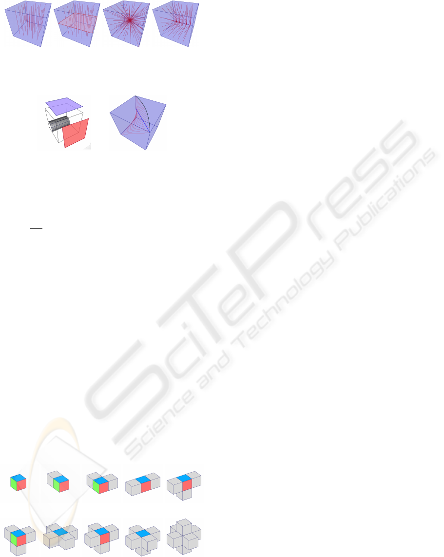
(a) (b) (c) (d)

Figure 2: The four types of projections we consider inside

each cell: (a) parallel, (b) planar, (c) perspective, (d) axial.

Figure 3: The axial parameterization maps straight line seg-

ments onto planar curves. A sample case using axial pro-

jection from the bottom back edge onto two external faces

(left); this projection maps the blue segment onto a planar

curve on the top face of the cubic cell (right).

P inside the cell will be projected along the direc-

tion CP.

• Axial projection: deﬁned by an axis a parallel to

one of the coordinate axes. For example, points

on an axis parallel to the X axis has points with

the form (λ, a

) for some λ ∈ R. A point P

inside the cell will be projected along the direction

(λ,P

− a

In all cases points inside the cell are projected onto

the cell’s faces. The ﬁrst three types of projections de-

ﬁne linear mappings, projecting mesh triangles inside

the cell onto triangles on the support plane of each

domain face, whereas the last projection type leads to

a non-linear mapping, projecting mesh triangles onto

triangular patches with curved edges (Figure 3). This

non-linearity property poses no problem to the ren-

dering algorithm, as discussed below.

Each parameterization is local to a cell c in the

sense that each G cell has a single projection type, and

only the geometry inside a G cell is projected onto its

domain faces. We now discuss, for each base case, the

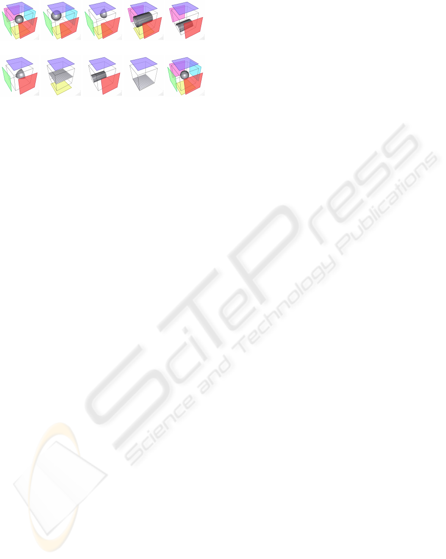
Case 0 Case 1 Case 2a Case 2b Case 3a

Case 3b Case 4a Case 4b Case 5 Case 6

Figure 4: Conﬁgurations of a G cells can be grouped into

the ten base cases shown. For each case we show a G cell

(with colored faces) and its non-empty 6-connected cells.

type of projection we use, which constraints affect the

parameter (~v,C,Π,a) controlling the projection (so as

to guarantee that points inside the cell are projected

only onto its domain faces), and how to compute a

suitable value for that parameter (Figure 5).

Case 0. All six faces are external. We use a perspec-

tive projection with the CoP C being any point in-

side the cell. This point can be computed simply

as the cell’s center.

Case 1. All faces are external except for one internal

face F. We also use a perspective projection, this

time C being any point on F. Our current imple-

mentation computes C as the middle point of F.

Case 2a. All edges are shared by external faces, ex-

cept for one internal edge e. Again, we use per-

spective projection with C being any point on e.

Our implementation uses the middle point of e.

Case 2b. Only two internal faces F

in opposite

directions. We use an axial projection, taking any

axis deﬁned joining a point on F

with a point on

. Our current implementation uses the axis de-

ﬁned by joining the middle points of F

and F

Case 3a. Three external faces and only two internal

edges e

. We also use an axial projection, with

the axis deﬁned by joining a point on e

and a

point on e

. Our current implementation simply

uses the midpoints of e

and e

Case 3b. Three internal faces meeting at a vertex v.

We use perspective projection from v.

Case 4a. This case is the complementary of case 2b,

with two parallel external faces F

. We use a

planar projection with Π being a plane parallel to

and F

. Our current implementation uses the

plane going through the cell’s center.

Case 4b. This case is the complementary of case 2a,

with a single external edge e

. For this case we

use the axial projection provided by the opposite

edge in the cell.

Case 5. This case is the complementary of case 1,

with a single external face F. We use a parallel

projection with ~v being the normal of F.

Case 6. This case, which is the complementary of

case 0, is handled using the same perspective pro-

jection.

3.3 Construction

We ﬁrst assume that a given grid resolution N has

been ﬁxed and discuss how to compute the G cells

of the resulting N × N × N grid (Section 3.3.1), and

how to sample properties to build the texture using the

GRAPP 2010 - International Conference on Computer Graphics Theory and Applications

184

Case 0 Case 1 Case 2a Case 2b Case 3a

Case 3b Case 4a Case 4b Case 5 Case 6

Figure 5: Projection type for each basic G cell conﬁgura-

tion. Points inside each G cell are projected onto the col-

ored faces using projection lines perpendicular to the shown

spherical/cylindrical/planar surface.

projections described above (Section 3.3.2). Then, a

simple algorithm for choosing a proper value for N is

presented in Section 3.3.3.

3.3.1 Computing the G Cells

This step simply accounts for dividing the bound-

ing cube of the input mesh M into an N × N × N

grid, and classifying the resulting cubic cells as W,

G or B. This can be done either in the CPU, follow-

ing the discretization algorithm described in (Andujar

et al., 2002), or in the GPU, using a voxelization algo-

rithm (Eisemann and Décoret, 2008). Our current im-

plementation uses the CPU-based approach because

it also provides, for each G cell, the list of faces inter-

secting it, which greatly accelerates the sampling of

surface attributes discussed below.

3.3.2 Sampling Surface Properties

We now describe a GPU-based algorithm for sam-

pling surface properties to ﬁll the 2D texture associ-

ated with each domain face. The algorithm traverses

all G cells {c

} and all the domain faces of each c

The basic idea is to render the geometry inside the

cell onto a texture, using a shader for computing the

projection.

The CPU-based part of the rendering algorithm

proceeds through the following steps:

1. Setup a frame buffer object (FBO) and a viewport

transformation matching the desired texture size.

2. Setup an orthographic camera facing the domain

face c

to be sampled.

3. Set the uniform variables encoding the cubic cell

and its projection type, to make this information

available to the geometry and fragment shaders.

4. Draw the mesh triangles intersecting the cell.

The vertex shader leaves the input vertices untrans-

formed, the projection being performed in a geome-

try shader. We have adopted this solution because,

due to the non-linearity of the mapping used for cases

2b, 3a and 4b, mesh triangles must be tessellated by

subdividing large mesh edges prior to projecting its

vertices. The geometry shader thus performs these

steps:

1. If the current cell uses axial projection (cases 2b,

3a, 4b), tessellate the triangle by uniformly subdi-

viding the edges longer than a user-deﬁned thresh-

old.

2. Use the projection type to project the vertices into

the support plane of the domain face c

to be ﬁlled.

For mesh triangles whose projection spans multi-

ple domain faces, some projected vertices might

lie outside the domain face, but OpenGL’s clip-

ping will take care of these cases.

3. For each primitive, emit the projected vertices, en-

coding its original position as texture coordinates.

Finally, the fragment shader simply encodes in the

output color the attribute to be sampled. Dis-

tance maps simply encode the distance between mesh

points P = (x, y, z) and their projection P

= (x

Note that these distances must be computed on a per-

fragment basis, as they do not interpolate linearly

when using e.g. perspective projection (cases 0, 1,

2a, 3b, Figure 5). Since the mapping is non-bijective,

multiple surface points might project onto the same

texel. In these cases the texel must encode the dis-

tance to the closest surface point. This is accom-

plished by simply setting the fragment depth to the

computed distance, so that OpenGL’s depth test will

discard occluded samples. Other surface signals such

as color and normal data are sampled in a similar way

(Figure 6).

3.3.3 Choosing a Proper Grid Size

A ﬁne grid provides a better approximation of the sur-

face mesh, each G cell having a simpler region inside

and thus more likely to be represented faithfully by

the distance maps. However, increasing the number

of cells also increases storage space and adds some

overhead to the rendering algorithm. Our algorithm

for choosing a proper grid resolution N strives to min-

imize the number of surface elements that map onto

the same texel. A simple estimation for this number

can be computed by running the sampling algorithm

above but using the stencil buffer to count the num-

ber of fragments projecting onto the same texel. So

we start with an 1 × 1 × 1 grid and compute the ratio

of occluded fragments. If the ratio is above a user-

RELIEF MAPPING ON CUBIC CELL COMPLEXES

185

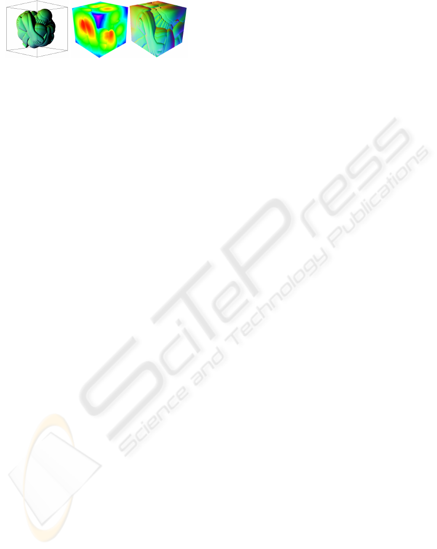
(a) (b) (c)

Figure 6: Sampling attribute values: (a) model inside a sin-

gle cubic cell; (b) sampled distance ||P−P

|| represented as

color temperature; (c) sampled normals.

deﬁned threshold, we increase (e.g. doubling) the res-

olution in each direction and repeat the above steps

until the ratio is below the threshold, or a maximum

max

is reached.

3.4 Representation

Our representation consists of:

• A lookup table encoding the G cells, and the pro-

jection type for each G cell.

• A collection of 2D textures (one for each domain

face) encoding the distance maps. Since all these

textures have the same size, they can be packaged

as an array texture (GL_EXT_texture_array ex-

tension). An array texture is accessed by shaders

as a single texture unit. A single layer is selected

using the r texture coordinate, and that layer is

then accessed as though it were a 2D texture us-

ing (s,t) coordinates.

• An array texture for each additional surface signal

(color, normal).

3.5 Rendering

Our representation can be rendered using both a direct

approach which reconstructs a triangle mesh approxi-

mating the object on-the-ﬂy, or a raycasting approach

which relies on intersecting viewing rays with the dis-

tance maps.

3.5.1 Geometry-based Rendering

Our representation can be rendered by reconstructing

a triangle mesh on the ﬂy using an algorithm similar

to that of Geometry Images (Gu et al., 2002). The

idea is to visit all texels of the distance maps and cre-

ate a pair of triangles for each 2x2 group of texels.

Each texel (u,v) of a domain face is associated with a

point P

= (x

) on the surface of a G cell, which

can be computed by a simple transformation from lo-

cal to global coordinates. Using the distance d stored

at texel (u, v) and the projection type of the G cell,

we can unproject point P

to get a point of the surface

mesh. Level-of-detail rendering is implemented by

mip-mapping the distance maps. During rendering,

the normal-map signal is rasterized over the triangles

by hardware, using bilinear ﬁltering of each quad in

the normal map. This reconstruction type allows our

representation to have similar uses than geometry im-

ages.

3.5.2 Raycasting Rendering

A more interesting feature of our representation is the

output-sensitive rendering through raycasting. Re-

lief mapping (Policarpo et al., 2005) can be easily

generalized to compute the intersection of a ray with

the surface implicitly encoded by distance maps built

from arbitrary projections. The classic approach for

relief mapping is to compute the ray-heightﬁeld in-

tersection by sampling points along the ray, ﬁrst us-

ing linear search to ﬁnd a sample inside the object,

and then reﬁning the intersection point through bi-

nary search, Figure 7(a). For each sampled point,

the height of the sample is compared with the depth

stored in the relief map to determine whether the sam-

ple is inside or outside the heightﬁeld. This idea

can be trivially extended from heightﬁelds to distance

maps constructed from the projection types discussed

in Section 3.2. We also sample points P

along the ray,

see Figure 7(b). Each sample P

is projected onto the

corresponding domain face to compute the projected

point P

which is converted to local (u

) coordi-

nates. The distance value d stored at (u

) is dequan-

tized and then compared with the distance ||P

− P

to check whether the sampled point is inside or out-

side the object. The distribution of tasks between the

different processors is as follows.

The CPU-based part of the rendering algorithm

proceeds through the following steps:

1. Bind the array textures encoding dis-

tance/color/normal maps to different texture

units, and bind also the texture encoding the LUT

of cubic cells and projection types to another

texture unit.

2. Draw the frontfaces of the G cells, just to ensure

that a fragment will be generated for any viewing

ray intersecting the underlying object.

The vertex shader performs no signiﬁcant computa-

tions. The most relevant part of the rendering relies

on the fragment shader, which performs these steps:

1. Compute the viewing ray.

2. Sample points on the ray using linear search to

ﬁnd the ﬁrst sample, if any, inside the object. For

GRAPP 2010 - International Conference on Computer Graphics Theory and Applications

186

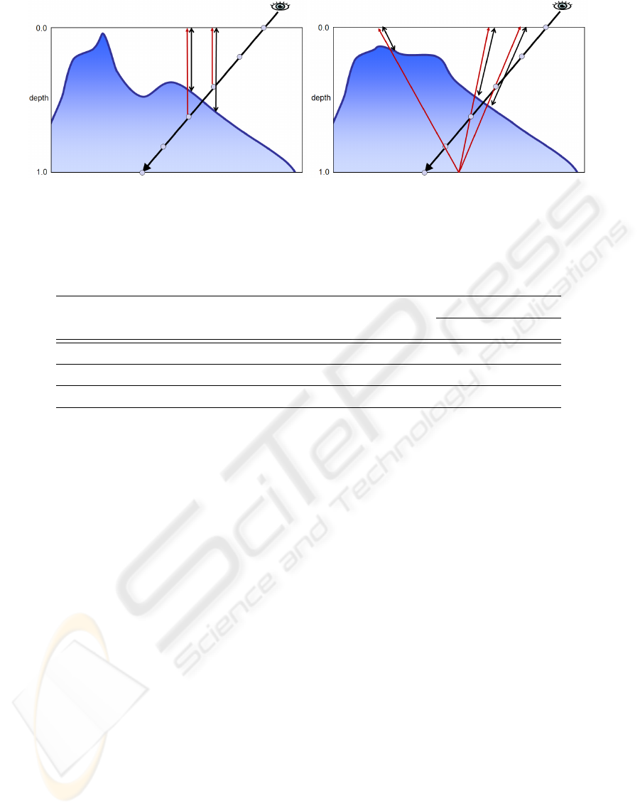
(a) (b)

Figure 7: Computing ray-surface intersections by sampling points along the ray: (a) surface encoded as a heightﬁeld (b)

surface encoded using a perspective projection. The red arrows indicate the direction of projection; black arrows show the

distance stored in the texture, which is checked against the real distance from the sampled point on ray to the projection plane.

Table 1: Construction times for the test models.

# Faces # G cells # Domain Texture Total Construction times

faces size size G cells Sampling

Egea 16.5K 18 42 64x64 336KB < 1s < 1s

Squirrel 20K 18 42 64x64 336KB < 1s < 1s

Moai 20K 20 48 64x64 384KB < 1s < 1s

Pensatore 1M 1 6 128x128 192KB 2 s 3 s

each sample point, we identify the cell c contain-

ing the sample, retrieve the projection P associ-

ated with the cell, and apply P to project the sam-

ple onto domain face. Stop as soon as a sample

inside the object is found. Otherwise, the ray does

not intersect the surface and hence the fragment is

discarded.

3. Reﬁne the intersection point using binary search,

as in classic relief mapping.

4. Use the texture coordinates (u, v) at the intersec-

tion point to lookup surface signals such as color

and normal data.

Most acceleration methods for relief mapping can be

also adopted to our approach. In particular, interval

mapping can be integrated into our approach with lit-

tle effort.

4 RESULTS

We have implemented a prototype version of the pro-

posed algorithms and we have tested them with de-

tailed models from the Aim@Shape repository.

Table 1 shows full construction times, including

the computation of the cells intersected by the mesh

and the sampling process required to build the dis-

tance and normal maps. Note that these times are

highly competitive and clearly outperform construc-

tion times of state-of-the-art parameterization algo-

rithms. The storage space required to store the array

textures has been computed using 2 bytes to quantize

distance values (Table 1). In all cases a low-resolution

grid was enough to obtain a parameterization with lit-

tle or no overlap between mesh triangles.

Figure 8 shows the results of our raycasting ren-

dering algorithm. Note that differences are hardly

noticeable. Rendering times measured on an Nvidia

GTX 280 are shown in Table 2. Rendering times are

clearly dominated by the number of fragments to be

processed. How these rendering times compare to

rendering the input model depends basically on the

complexity of the model and its screen projection.

Simple models with large screen projections are ren-

dered much faster using the original mesh, whereas

complex models with small screen projection render

much faster with our output-sensitive approach. Ta-

ble 2 also shows the number of ray intersections that

can be computed per second. It is worth to remark

that the ray throughput we achieve also holds for re-

ﬂected and refracted rays. The rendering time for

drawing the model as is or its reﬂection on a curved

mirror is roughly proportional to the number of ray in-

tersections. This unique feature makes our approach

RELIEF MAPPING ON CUBIC CELL COMPLEXES

187

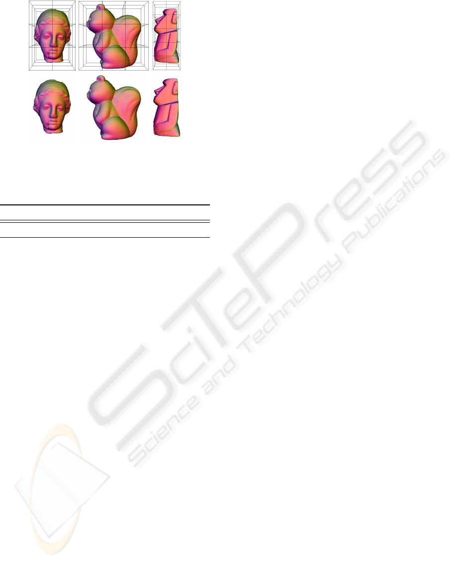
Figure 8: Results using raycasting rendering (bottom row)

compared with the original model (top row)

Table 2: Rendering times using raycasting on a 512x512

viewport, and number of ray-surface intersections.

Egea Squirrel Moai Pensatore

Frame rate 107 fps 112 fps 99 fps 111 fps

Rays/s 28M 29M 26M 29M

particularly suitable for ray-tracing in the GPU. Note

that competing representations such as relief-mapped

meshes only perform well once the fragment coordi-

nates and interpolated texture coordinates have been

computing during the rasterization stage; otherwise,

additional spatial data structures are required to com-

pute the ray-mesh intersection.

Unlike polycube maps (Tarini et al., 2004), our

representation can be computed fully automatically.

Furthermore, since the parameterization is implicit

and quickly reversible from the distance maps, the

original mesh is not required to render the surface,

and the surface can be rendered efﬁciently using a

raycasting approach. The simplicity of our approach

comes at a price though. Since we leave out optimiza-

tion steps performed during construction of polycube

maps and the ﬂexibility offered by storing explicit

texture coordinates, our parameterization might suf-

fer from higher distortion.

5 CONCLUSIONS

The main contributions of the paper are (a) a

projection-based method for deﬁning implicit param-

eterization of surface meshes onto an automatically

computed set of cubic cells, (b) a uniﬁed representa-

tion of detailed meshes based on the above param-

eterization using array textures encoding projection

distances and other surface signals such as normals

and color, (c) an efﬁcient GPU-based algorithm for

sampling these signals, and (d) a rendering algorithm

which generalizes relief mapping to arbitrary projec-

tions. Since we target GPU-based construction and

rendering, we restrict ourselves to easily invertible,

implicit projections, at the expense of bijectivity and

distortion minimization guarantees. Our approach

is oriented towards arbitrarily-detailed models whose

main features are roughly well captured by a low res-

olution grid. Complex surfaces with many thin parts

such as bones or pipes might require a high resolution

grid to sample faithfully the surface, thus making our

approach less attractive for representing these models.

There are several directions that can be pursued

to extend the current work. The parameters deﬁning

each projection type can be optimized by taking into

account the distribution of the geometry inside each G

cell, at the expense of higher construction times. For

instance, the CoP used by case 0 can be computed as

the centroid of the part of the mesh intersecting the

cell, instead of taking just the cell’s center. We would

like to further compare our projection with the projec-

tor operator proposed by Tarini et al. (2004). Leaving

out further optimization steps, the projector operator

is also implicitly deﬁned as in our case. Another ob-

vious extension is to use an octree instead of equal-

sized cubic cells. The criteria for grid reﬁnement can

be applied for each octree node with little effort. This

would result in G cells at different levels and with dif-

ferent texture sizes. Since array textures require each

2D texture layer to have the same size, multiple array

textures will be needed, one for each different texture

size.

ACKNOWLEDGEMENTS

This work has been partially funded by the Span-

ish Ministry of Science and Technology under grant

TIN2007-67982-C02. All test models were provided

by the AIM@SHAPE Shape Repository.

REFERENCES

Andujar, C., Boo, J., Brunet, P., Fairen, M., Navazo,

I., Vazquez, P., and Vinacua, A. (2007). Omni-

directional relief impostors. Computer Graphics Fo-

rum, 26(3):553–560.

Andujar, C., Brunet, P., and Ayala, D. (2002). Topology-

reducing simpliﬁcation through discrete models. ACM

Transactions on Graphics, 20(6):88–105.

Baboud, L. and Décoret, X. (2006). Rendering geometry

with relief textures. In Proc. of Graphics Interface,

pages 195–201, Toronto, Canada.

GRAPP 2010 - International Conference on Computer Graphics Theory and Applications

188

Benson, D. and Davis, J. (2002). Octree textures. ACM

Transactions on Graphics (TOG), 21(3):785–790.

Dong, S., Bremer, P.-T., Garland, M., Pascucci, V., and

Hart, J. C. (2006). Spectral surface quadrangulation.

ACM Transactions on Graphics, 25(3):1057–1066.

Donnelly, W. (2005). Per-pixel displacement mapping

with distance functions. In GPU Gems 2: Program-

ming Techniques for High-Performance Graphics and

General-Purpose Computation, pages 123–136.

Eisemann, E. and Décoret, X. (2008). Single-pass gpu solid

voxelization for real-time applications. In GI ’08:

Proceedings of graphics interface 2008, pages 73–80.

Floater, M. S. and Hormann, K. (2005). Surface parameter-

ization: a tutorial and survey. In N. A. Dodgson, M.

S. F. and Sabin, M. A., editors, Advances in Multireso-

lution for Geometric Modelling, Mathematics and Vi-

sualization, pages 157–186. Springer, Berlin.

García, I. and Patow, G. (2008). Igt: inverse geometric tex-

tures. ACM Transactions on Graphics, 27(5):1–9.

Gu, X., Gortler, S. J., and Hoppe, H. (2002). Geometry

images. ACM Transactions on Graphics, 21(3):355–

361.

Guskov, I., Vidim

ce, K., Sweldens, W., and Schröder, P.

(2000). Normal meshes. In SIGGRAPH’00, pages

95–102.

Lee, A. W. F., Sweldens, W., Schröder, P., Cowsar, L.,

and Dobkin, D. (1998). Maps: multiresolution adap-

tive parameterization of surfaces. In SIGGRAPH’98,

pages 95–104.

Lefebvre, S. and Dachsbacher, C. (2007). Tiletrees. In

Proceedings of the 2007 symposium on Interactive 3D

graphics and games, page 31. ACM.

Lefebvre, S., Hornus, S., and Neyret, F. (2005). Octree Tex-

tures on the GPU. GPU gems, 2:595–613.

Lefohn, A., Sengupta, S., Kniss, J., Strzodka, R., and

Owens, J. (2006). Glift: Generic, efﬁcient, random-

access GPU data structures. ACM Transactions on

Graphics (TOG), 25(1):60–99.

Losasso, F., Hoppe, H., Schaefer, S., and Warren, J. (2003).

Smooth geometry images. In SGP ’03: 2003 Eu-

rographics/ACM SIGGRAPH symposium on Geome-

try processing, pages 138–145. Eurographics Associ-

ation.

Peachey, D. (1985). Solid texturing of complex surfaces.

ACM SIGGRAPH Computer Graphics, 19(3):286.

Perlin, K. (1985). An image synthesizer. ACM SIGGRAPH

Computer Graphics, 19(3):296.

Policarpo, F. and Oliveira, M. M. (2006). Relief mapping

of non-height-ﬁeld surface details. In Proc. of ACM

Symp. on Interactive 3D Graphics and Games, pages

55–62.

Policarpo, F., Oliveira, M. M., and Comba, J. (2005). Real-

time relief mapping on arbitrary polygonal surfaces.

In Proc. of ACM Symposium on Interactive 3D Graph-

ics and Games, pages 155–162.

Praun, E., Sweldens, W., and Schröder, P. (2001). Con-

sistent mesh parameterizations. In SIGGRAPH ’01,

pages 179–184.

Purnomo, B., Cohen, J. D., and Kumar, S. (2004). Seam-

less texture atlases. In SGP ’04: Proceedings of the

2004 Eurographics/ACM SIGGRAPH symposium on

Geometry processing, pages 65–74.

Sheffer, A., Praun, E., and Rose, K. (2006). Mesh param-

eterization methods and their applications. Founda-

tions and Trends in Computer Graphics and Vision,

2(2):105–171.

Tarini, M., Hormann, K., Cignoni, P., and Montani, C.

(2004). Polycube-maps. In SIGGRAPH ’04 , pages

853–860.

Tatarchuk, N. (2006). Dynamic parallax occlusion mapping

with approximate soft shadows. In I3D ’06: Proceed-

ings of the 2006 symposium on Interactive 3D graph-

ics and games, pages 63–69.

RELIEF MAPPING ON CUBIC CELL COMPLEXES

189